Linear Dimensionality Reduction

主要包括主成分分析（PCA）和经典相关分析（CCA）的推导

Outline:

• Introduction
• Principal Component Analysis
• Canonical Variate and Correlation Analysis

7.1 Introduction

Target: find a projection that project data onto a lower-dimensional subspace without losing important information.

• One possible way to accomplish this is through feature selection.
• Another way is by creating a reduced set of transformations(linear or nonlinear) of the input variables, which is often referred to as feature extraction.

Principal Component Analysis(PCA) and Cononical Variate and Correlation Analysis(CVA/CCA) are linear methods that are most popular in use today. Both these mothods are eigenvalue-eigenvector problems and can be viewed as special cases of multivariate reduced-rank regression.

7.2 Principal Component Analysis

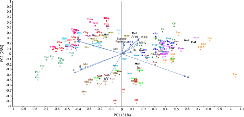
PCA was introduced as technique for deriving a reduced set of orthogonal linear projections of a single collection of correlated variables $X=(X_1,…,X_r)^T$, where the projections are oredered by decreasing variances. It’s also a method of decorrelating $X$.

Note: Variance is a second-order property of a random variable and is an important measurement of the amount of information in that variable.

How to make use of the principal component scores (in decreasing order):

• The first few ones: revealing whether most of the data actually live on a linear subspace of $\mathbb{R}^r$ and identifying outliers, distributional peculiarities and clusters of points.
• The last few ones: detect collinearity and outliers that pop up and alter the perceived dimensionality of the data (which has near-zero variance)

7.2.1 Population Principal Components

Assume that the ramdom $r$-vector $X=(X_1,…,X_r)^T$ has mean $\mu_X$ and $(r\times r)$ covariance matrix $\Sigma_{XX}$.

PCA: set of $r$ variables $X_r$ (unordered and correlated) $\rightarrow$ set of $t$ variables $\xi_t$(ordered and uncorrelated), where $t<r$

First t principal components:

$$\xi_j = b_j^TX = b_{j1}X_1+...+b_{jr}X_r, j=1,2,...,t$$

where we minimize the loss of information due to replacement.(7.2.2,7.2.3)

We here interpreted “information” with the total variation of the original input variables:

$$\sum_{j=1}^r var(X_j)=tr(\Sigma_{XX})$$

From the spectral decomposition theorem, we can write

$$\Sigma_{XX}=U\Lambda U^T, U^TU=I_r$$

where the diagonal matrix $\Lambda$ has diagonal elements the eigenvalues $\left\{\lambda_j\right\}$ of $\Sigma_{XX}$, and the columns of $U$ are the eigenvectors of $\Sigma_{XX}$.

Thus, we obtain the total variation by

$$tr(\Sigma_{XX})=tr(\Lambda)=\sum_{j=1}^r\lambda_j$$

The $j$th coefficient vector $b_j=(b_{1j},…,b_{rj})^T$ is chosen so that:

• The first $t$ linear projections $\xi_j,j=1,2,…,t$ of $X$ are ranked in importance through their variances $\left\{var(\xi_j)\right\}$ that $var(\xi_1)\geq var(\xi_2)\geq …\geq var(\xi_t)$
• $\xi_j$ is uncorrelated with all $\xi_k,k<j$

There are two popular derivations of the set of principal components of $X$:

• Least-Squares Optimality crieterion (analogous with regression)
• Variance-maximizing technique

7.2.2 Least-Squares Optimality of PCA

Let

$$B=(b_1,...,b_t)^T$$

be a $(t\times r)$-matrix of weights ($t\leq r$), then the linear projections can be written as

$$\xi = BX$$

where $\xi=(\xi_1,…,\xi_t)^T\in\mathbb{R}^{t\times n}$. Note that $X\in\mathbb{R}^{r\times n}$ is the observations matrix with variables as rows and individual observations as columns.

We want to find a $r$-vector $\mu$ and an ($r\times t$)-matrix $A$ such that

$$X\approx \mu+A\xi$$

(用 $X$ 对 $\xi$ 回归，类似“压缩”后“还原”的思想，通过“还原”后与原本数据的误差来评估“压缩器”的好坏)

Here we use least-squares error criterion to find the optimum $\mu,A$:

$$E[(X-\mu-A\xi)^T(X-\mu-A\xi)]$$

recall that we have $\xi=BX$, we can write

$$E[(X-\mu-ABX)^T(X-\mu-ABX)]$$

When $t=1$, the least-squares problem is equivalent to

$$\min_{\mu,A,B}E\sum_{j=1}^r(X_j-\mu_j-a_{j1}b_1^TX)^2$$

where $X=(X_1,…,X_r)^T,\mu=(\mu_1,…,\mu_r)^T,A=a_1=(a_{11},…,a_{r1})^T$, and $B=b_1^T$

For $t>1$, the criterion is similar to Weighted Sum-of-Squares Criterion with $Y\equiv X,s=r,\Gamma=I_r$. Hence, the minimum solution is obtained by reduced-rank regression

$$A^{(t)}=(v_1,...,v_t)=B^{(t)T}, \mu^{(t)}=(I_r-A^{(t)}B^{(t)})\mu_X$$

where $v_j=v_j(\Sigma_{XX})$ is the eigenvector associated with the $j$th largest eigenvalue of $\Sigma_{XX}$ (i.e.$\lambda_j$).

Thus, our best rank-$t$ approximation to the original $X$ is given by

$$\hat{X}^{(t)}=\mu^{(t)}+C^{(t)}X=\mu_X+C^{(t)}(X-\mu_X)$$

where

$$C^{(t)}=A^{(t)}B^{(t)}=\sum_{j=1}^t v_jv_j^T$$

is the reduced-rank regression coefficient matrix with rank $t$ for the principal components case.

The minumum of $E[(X-\mu-ABX)^T(X-\mu-ABX)]$ is given by $\sum_{j=t+1}^r \lambda_j$.

The first $t$ principal components of $X$ are given by

$$\xi_j=v_j^TX$$

and the covariance between $\xi_i$ and $\xi_j$ is

$$cov(\xi_i,\xi_j)=v_i^T\Sigma_{XX}v_j=v_i^T\lambda_jv_j=\delta_{ij}\lambda_j$$

7.2.3 PCA as a Variance-Maximization Technique

In the original derivation of principal components, the coefficient vectors

$$b_j=(b_{j1},...,b_{jr})^T,j=1,2,...,t$$

were chosen in a sequential manner so that:

• $var(\xi_j)=b_j^T\Sigma_{XX}b_j$ are arranged in descending order subject to the normalizations $b_j^Tb_j=1,j=1,…,t$
• $cov(\xi_i,\xi_j)=b_i^T\Sigma_{XX}b_j=0,i<j$

The first principal component $\xi_1$ is obtained by choosing the $r$ coefficients $b_1$ for the linear projection $\xi_1$ (subject to normalization). A unique choice of $\left\{\xi_j\right\}$ is obtained through the normalization constraint $b_j^Tb_j=1,j=1,…,t$

$$\begin{aligned} f(b_1)&=var(\xi_1)+\lambda_1(1-b_1^Tb_1)\\ &=b_1^T\Sigma_{XX}b_1+\lambda_1(1-b_1^Tb_1) \end{aligned}$$

where $\lambda_1$ is a Lagrangian multiplier.

$$\frac{\partial f(b_1)}{\partial b_1}=2(\Sigma_{XX}-\lambda_1I_r)b_1\overset{set}{=}0$$

We require $b_1\neq{0}$, so $|\Sigma_{XX}-\lambda_1I_r|=0$.

Note that when $\lambda_1$ is the largest eigenvalue of $\Sigma_{XX}$, let $b_1$ be the relevant eigenvector. We have $\Sigma_{XX}b_1=\lambda_1b_1$ hence $|\Sigma_{XX}-\lambda_1I_r|=0$.

Why has to be the largest?

• If not, $var(\xi_1)=b_1^T\Sigma_{XX}b_1=\lambda_1b_1^Tb_1=\lambda_1$ is not the largest case.

Similarly, the second principal component $\xi_2$ and coefficients $b_2$ are chosen. That is, maximize $var(\xi_2)=b_2^T\Sigma_{XX}b_2$ subject to $b_2^Tb_2=1$ and $b_1^Tb_2=0$

$$f(b_2)=b_2^T\Sigma_{XX}b_2-\lambda_2(1-b_2^Tb_2)+\mu b_1^Tb_2$$

where $\lambda_2,\mu$ are Lagrangian multipliers.

$$\frac{\partial f(b_2)}{\partial b_2}=2(\Sigma_{XX}-\lambda_2I_r)b_2+\mu b_1\overset{set}{=}0$$

Premultiplying $b_1^T$ then

$$2b_1^T\Sigma_{XX}b_2+\mu=0$$

Premultiplying $(\Sigma_{XX}-\lambda_1I_r)b_1=0$ by $b_2^T$ yields $b_2^T\Sigma_{XX}b_1=0$, whence $\mu=0$.

This means that $\lambda_2$ is the second largest eigenvalue of $\Sigma_{XX}$ and $b_2$ is the relevant eigenvector.

In this sequential manner, we obtain the remaining sets of coefficients for the principal components.

Matrix form:

$$f(B)=var(\xi)+\lambda(BB^T-1)=B\Sigma_{XX}B^T-\lambda(BB^T-1)$$ $$\frac{\partial f}{\partial B}=2\Sigma_{XX}B-2\lambda B\overset{set}{=}0$$ $$\Leftrightarrow \Sigma_{XX}B=\lambda B$$

7.2.4 Sample Principal Components

We estimate the principal components of $X$ using a random sample with observed values $\left\{x_i\right\}$

$$\hat{\mu}_X=\bar{x}=\frac{1}{n}\sum_{i=1}^n x_i$$

Let $x_{ci}=x_i-\bar{x}$ and $X_c=(x_{c1},…,x_{cn})$ we estimate $\Sigma_{XX}$ by

$$\hat{\Sigma}_{XX}=\frac{1}{n}X_cX_c^T$$

The ordered eigenvalues of $\hat{\Sigma}_{XX}$ are denoted by $\hat{\lambda}_1\geq\hat{\lambda}_2\geq…\geq\hat{\lambda}_r\geq 0$ and the relevent eigenvector $\hat{v}_j$.

Then we estimate $A^{(t)}$ and $B^{(t)}$ by

$$\hat{A}^{(t)}=(\hat{v}_1,...,\hat{v}_t)=\hat{B}^{(t)T}$$

The best rank-$t$ reconstruction of $X$ is given by

$$\hat{x}^{(t)}=\bar{x}+\hat{C}^{(t)}(x-\bar{x})$$

where

$$\hat{C}^{(t)}=\hat{A}^{(t)}\hat{B}^{(t)}=\sum_{j=1}^t\hat{v}_j\hat{v}_j^T$$

is the reduced-rank regression coefficient matrix.

The $j$th sample PC score is given by

$$\hat{\xi}_j=\hat{v}_j^TX_c=\hat{v}_j^T(X-\bar{X})$$

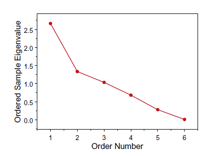
7.2.5 Selection of the number of components

Scree Plot: The sample eigenvalues from a PCA are ordered from largest to smallest. (Find the “elbow”)

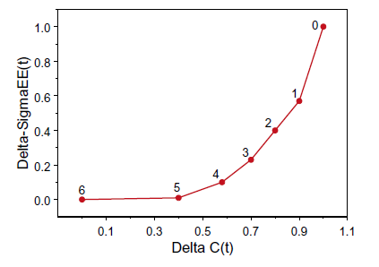
PC Rank Trace: Obtain a useful estimate of the rank of the regression coefficient matrix $C$.

$$\Delta\hat{C}^{(t)}=(1-\frac{t}{r})^{1/2}$$ $$\Delta\hat{\Sigma}_{\epsilon\epsilon}^{(t)}=(\frac{\hat{\lambda}_{t+1}^2+...+\hat{\lambda}_r^2}{\hat{\lambda}_1^2+...+\hat{\lambda}_r^2})^{1/2}$$

A plot of $\Delta\hat{\Sigma}_{\epsilon\epsilon}^{(t)}$ against $\Delta\hat{C}^{(t)}$ is the PC rank trace plot.(Find the “elbow”)

Kaiser’s Rule: Only those eigenvalues exceed 1 would be retained. (too controversial)

7.2.6 Invariance and Scaling

Note that the principal components are NOT invariant under rescalings of the initial variables. (sensitive to the units of measurement of the different input variables)

One possible way to solve this is to rescale the input data

$$Z\leftarrow(diag\left\{\hat{\Sigma}_{XX}\right\})^{-1/2}(X-\hat{\mu}_X)$$

which is equivalent to carrying out PCA using the correlation matrix (rather than the covariance matrix).

7.2.7 What can be gained from using PCA

• decorrelate the original variables
• carry out data compression
• reconstruct the original input data using a reduced number of variables according to a least-squares criterion
• identify potential clusters in the data.

PCA can be misleading when there are outliers in the data, or the linearity of PCA fits badly to the data.

7.3 Canonical Variate and Correlation Analysis

7.3.1 Canonical Variates and Canonical Correlations

Assume that

$$\left( \begin{matrix} X\\Y \end{matrix} \right)$$

is a collection of $r+s$ variables partitioned into two disjoint subcollections, where $X$ and $Y$ are jointly distributed with mean vector and covariance matrix given by

$$E\left\{\left(\begin{matrix}X\\Y\end{matrix}\right)\right\}=\left(\begin{matrix}\mu_X\\\mu_Y\end{matrix}\right)$$ $$E\left\{\left(\begin{matrix}X-\mu_X\\Y-\mu_Y\end{matrix}\right)\left(\begin{matrix}X-\mu_X\\Y-\mu_Y\end{matrix}\right)^T\right\}=\left(\begin{matrix}\Sigma_{XX}&\Sigma_{XY}\\\Sigma_{YX}&\Sigma_{YY}\end{matrix}\right)$$

CVA seeks to replace the two sets of correlated variables by $t$ pairs of new variables

$$(\xi_i,\omega_i),i=1,2,...,t,\quad t\leq\min(r,s)$$

where

$$\begin{cases} \xi_j=g_j^TX=g_{1j}X_1+...+g_{rj}X_r\\ \omega_j=h_j^TY=h_{1j}Y_1+...+h_{sj}Y_s \end{cases}$$

The $j$th pairs of coefficient vectors are chosen so that

• the pairs are ranked in importance through their correlations that $\rho_1\geq…\geq\rho_t$ $$\rho_j=corr(\xi_j,\omega_j)=\frac{g_j^T\Sigma_{XY}h_j}{(g_j^T\Sigma_{XX}g_j)^{1/2}(h_j^T\Sigma_{YY}h_j)^{1/2}}$$
• $cov(\xi_j,\xi_k)=g_j^T\Sigma_{XX}g_k=0,k<j.$
• $cov(\omega_j,\omega_k)=h_j^T\Sigma_{XX}h_k=0,k<j.$

The paris are known as the first $t$ pairs of canonical variates of $X$ and $Y$ and their correlations as the $t$ largest canonical correlations.

7.3.2 Least-Squares Optimality of CVA

Let the $(t\times r)$-matrix $G$ and the $(t\times s$-matrix $H$, with $1\leq t\leq\min(r,s)$ be such that $X$ and $Y$ are linearly projected

$$\xi=GX,\quad\omega=HY$$

Consider the problem of finding $\nu,G,H$ so that

$$HY\approx\nu+GX$$

which minimize the $(t\times t)$-matrix

$$E\left\{(HY-\nu-GX)(HY-\nu-GX)^T\right\}$$

where we assume that the covariance matrix of $\omega$ is $\Sigma_{\omega\omega}=H\Sigma_{YY}H^T=I_t$

According to the Poincaré Separation Theorem, the cirterion is minimize when the coloumns of $U$ are the eigenvectors relevent to the first $t$ eigenvalues of $R$. (see Section 3.2.10)

Some conditions when the inequalities become equalities:

$$\nu=H\mu_Y-G\mu_X$$ $$G=\Sigma_{\omega X}\Sigma_{XX}^{-1}=H\Sigma_{YX}\Sigma_{XX}^{-1}$$ $$U^T=H\Sigma_{YY}^{1/2},\quad U^TU=I_t$$ $$R=\Sigma_{YY}^{-1/2}\Sigma_{YX}\Sigma_{XX}^{-1}\Sigma_{XY}\Sigma_{YY}^{-1/2}$$

To summarize:

$$\nu^{(t)}=H^{(t)}\mu_Y-G^{(t)}\mu_X$$ $$G^{(t)}=\left(\begin{matrix}v_1^T\\ \vdots \\ v_t^T\end{matrix}\right)\Sigma_{YY}^{-1/2}\Sigma_{YX}\Sigma_{XX}^{-1}=\left(\begin{matrix}\lambda_1u_1^T\\ \vdots \\ \lambda_tu_t^T\end{matrix}\right)\Sigma_{XX}^{-1/2}$$ $$H^{(t)}=\left(\begin{matrix}v_1^T\\ \vdots \\ v_t^T\end{matrix}\right)\Sigma_{YY}^{-1/2}$$

where $u_j$ is the eigenvector relevent to the $j$th largest eigenvalue $\lambda_j^2$ of

$$R^*=\Sigma_{XX}^{-1/2}\Sigma_{XY}\Sigma_{YY}^{-1}\Sigma_{YX}\Sigma_{XX}^{-1/2}$$

and $v_j$ is the eigenvector relevent to the $j$th largest eigenvalue $\lambda_j^2$ of

$$R=\Sigma_{YY}^{-1/2}\Sigma_{YX}\Sigma_{XX}^{-1}\Sigma_{XY}\Sigma_{YY}^{-1/2}$$

The $jth$ pair of canonical variates socres is given by

$$\xi_j=g_j^TX,\quad\omega_j=h_j^TY$$

where

$$g_j=\Sigma_{XX}^{-1}\Sigma_{XY}\Sigma_{YY}^{-1/2}v_j=\lambda_j\Sigma_{XX}^{-1/2}u_j$$ $$h_j=\Sigma_{YY}^{-1/2}v_j$$

7.3.3 CVA as a Correlation-Maximization Technique

Consider the linear poojections

$$\xi=g^TX,\quad\omega=h^TY$$

Assume that $E(X)=\mu_X=0,E(Y)=\mu_Y=0$ and $g^T\Sigma_{XX}g=1,h^T\Sigma_{YY}h=1$.

We try to maximize the correlation

$$corr(\xi,\omega)=g^T\Sigma_{XY}h$$

The problem is equivalent to maximize

$$f(g,h)=g^T\Sigma_{XY}h-\frac{1}{2}\lambda(g^T\Sigma_{XX}g-1)-\frac{1}{2}\mu(h^T\Sigma_{YY}h-1)$$

where $\lambda,\mu$ are Lagrangian multipliers.

$$\begin{cases} \frac{\partial f}{\partial g}=\Sigma_{XY}h-\lambda\Sigma_{XX}g\overset{set}{=}0\\ \frac{\partial f}{\partial h}=\Sigma_{YX}g-\mu\Sigma_{YY}h\overset{set}{=}0 \end{cases}$$

First, premultiplying $g^T$ and $h^T$ respectively, we have

$$\begin{cases} g^T\Sigma_{XY}h-\lambda g^T\Sigma_{XX}g=0\\ h^T\Sigma_{YX}g-\mu h^T\Sigma_{YY}h=0 \end{cases}$$

whence, the correlation between $\xi$ and $\omega$ satisfies

$$g^T\Sigma_{XY}h=\lambda=\mu$$

Hence, the original problem is equivalent to maximize the Lagrangrian multipliers.

Eigen-decomposition method:

Premultiplying $\Sigma_{XX}^{-1}$ and $\Sigma_{YY}^{-1}$ respectively

$$\begin{cases} \Sigma_{XX}^{-1}\Sigma_{XY}h-\lambda g=0\\ \Sigma_{YY}^{-1}\Sigma_{YX}g-\lambda h=0 \end{cases}$$

Rearrange the two equalities

$$\begin{cases} \Sigma_{XX}^{-1}\Sigma_{XY}\Sigma_{YY}^{-1}\Sigma_{YX}g=\lambda^2 g\\ \Sigma_{YY}^{-1}\Sigma_{YX}\Sigma_{XX}^{-1}\Sigma_{XY}h=\lambda^2 h \end{cases}$$

It can be shown that $g$ and $h$ are respectively chosen by the eigenvectors of

$$\begin{cases} N=\Sigma_{XX}^{-1}\Sigma_{XY}\Sigma_{YY}^{-1}\Sigma_{YX}\\ N^*=\Sigma_{YY}^{-1}\Sigma_{YX}\Sigma_{XX}^{-1}\Sigma_{XY} \end{cases}$$

To maximize $\lambda$, choose the eigenvectors relevant to the largest $t$ eigenvalues of $N,N^*$.

Least-square form:

Premultiplying $\Sigma_{YX}\Sigma_{XX}^{-1}$ to $\Sigma_{XY}h-\lambda\Sigma_{XX}g=0$ we have

$$\Sigma_{YX}\Sigma_{XX}^{-1}\Sigma_{XY}h=\lambda\Sigma_{YX}g$$

Recall that $\Sigma_{YX}g-\mu\Sigma_{YY}h=0$, we have

$$\Sigma_{YX}\Sigma_{XX}^{-1}\Sigma_{XY}h=\lambda\mu\Sigma_{YY}h$$ $$\Leftrightarrow (\Sigma_{YX}\Sigma_{XX}^{-1}\Sigma_{XY}-\lambda^2\Sigma_{YY})h=0$$

For there to be a nontrival solution, the following determinant has to be zero

$$|\Sigma_{YX}\Sigma_{XX}^{-1}\Sigma_{XY}-\lambda^2\Sigma_{YY}|=0$$ $$\Leftrightarrow |\Sigma_{YY}^{-1/2}\Sigma_{YX}\Sigma_{XX}^{-1}\Sigma_{XY}\Sigma_{YY}^{-1/2}-\lambda^2I_s|=0$$

It can be shown that the determinant above is a polynomial in $\lambda^2$ of degree $s$, having $s$ real roots $\lambda_1^2\geq\lambda_2^2\geq…\geq\lambda_s^2\geq 0$, which are the ordered eigenvalues of

$$R=\Sigma_{YY}^{-1/2}\Sigma_{YX}\Sigma_{XX}^{-1}\Sigma_{XY}\Sigma_{YY}^{-1/2}$$

with relevant eigenvectors $v_1,…,v_s$.

The resultant choice of $g$ and $h$ are given by

$$g_1=\Sigma_{XX}^{-1}\Sigma_{XY}\Sigma_{YY}^{-1/2}v_1,\quad h_1=\Sigma_{YY}^{-1/2}v_1$$

Then the pairs are

$$\xi_1=g_1^TX,\quad\omega_1=h_1^TY$$

and their correlation is

$$corr(\xi_1,\omega_1)=g_1^T\Sigma_{XY}h_1=\lambda_1$$

Then we choose the other projections in this sequential manner by adding constraint

$$g^T\Sigma_{XX}g_1=h^T\Sigma_{YY}h_1=0$$ $$corr(\xi,\omega_1)=g^T\Sigma_{XY}h_1=\lambda_1g^T\Sigma_{XX}g_1=0$$ $$corr(\omega,\xi_1)=h^T\Sigma_{YX}g_1=\lambda_1h^T\Sigma_{YY}h_1=0$$

Appendix A: Weighted Sum-of-Squares Criterion

#TODO