应用回归分析

应用回归分析课程内容整理，参考教材：Applied Linear Statistical Models 5e by Kutner

Chap1 Linear Regression with One Predictor Variable

Outline:

• Relations between variables
• Concepts in Regression Models
  • random error
  • residuals
• Simple Linear Regression Model with Distribution of Error Terms Unspecified
  • Least square estimators(LSEs)
  • Properties of LSEs
• Normal Error Regression Model

1.1 Relations between Variables

Functional Relation: $Y=f(X)$

Statistical Realtion: $Y=f(X)+\epsilon$

1.2 Concepts in Regression models

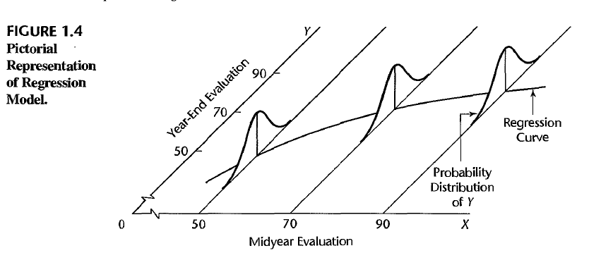
A regression model is a formal means of expressing the two essential ingredients of a statistical relation:

1. A tendency of the response variable $Y$ to vary with the predictor variable $X$ in a systematic fashion (There is a probability distribution of $Y$ for each level of $X$)
2. A scattering of points around the curve of statistical relationship (The means of these probability distributions vary in some systematic fashion with $X$)

$$Y=\alpha+\beta X+\epsilon,\quad\epsilon\sim N(0,\sigma^2)$$

Two distinct goals:

1. (Estimation) Understanding the relationship between predictor variables and response variables
2. (Prediction) Predicting the future response given the new observed predictors

Note: Always need to consider scope of the model, and statistical relationship generally does not imply causality.

1.3 Simple Linear Regression Model with Distribution of Error Terms Unspecified

$$Y_i=\beta_0+\beta_1 X_i+\epsilon_i,i=1,2,...,n$$

where $\epsilon_i\sim N(0,\sigma^2)$, $\epsilon_i$ and $\epsilon_j$ are uncorrelated. $X_i$ is a fixed known constant and $\beta_0,\beta_1,\sigma^2$ are unknown parameters.

The response $Y_i$ = deterministic term + random term, which implies that $Y_i$ is a random variable:

$$E(Y_i)=\beta_0+\beta_1 X_i,\quad Var(Y_i)=\sigma^2,\quad cov(Y_i,Y_j)=cov(\epsilon_i,\epsilon_j)=0$$

Alternative form:

$$Y_i=(\beta_0+\beta_1\bar{X})+\beta_1(X_i-\bar{X})+\epsilon_i$$

1.4 Data for Regression Analysis

• Obeservational Data
• Experimental Data
• Completely Randomized Design

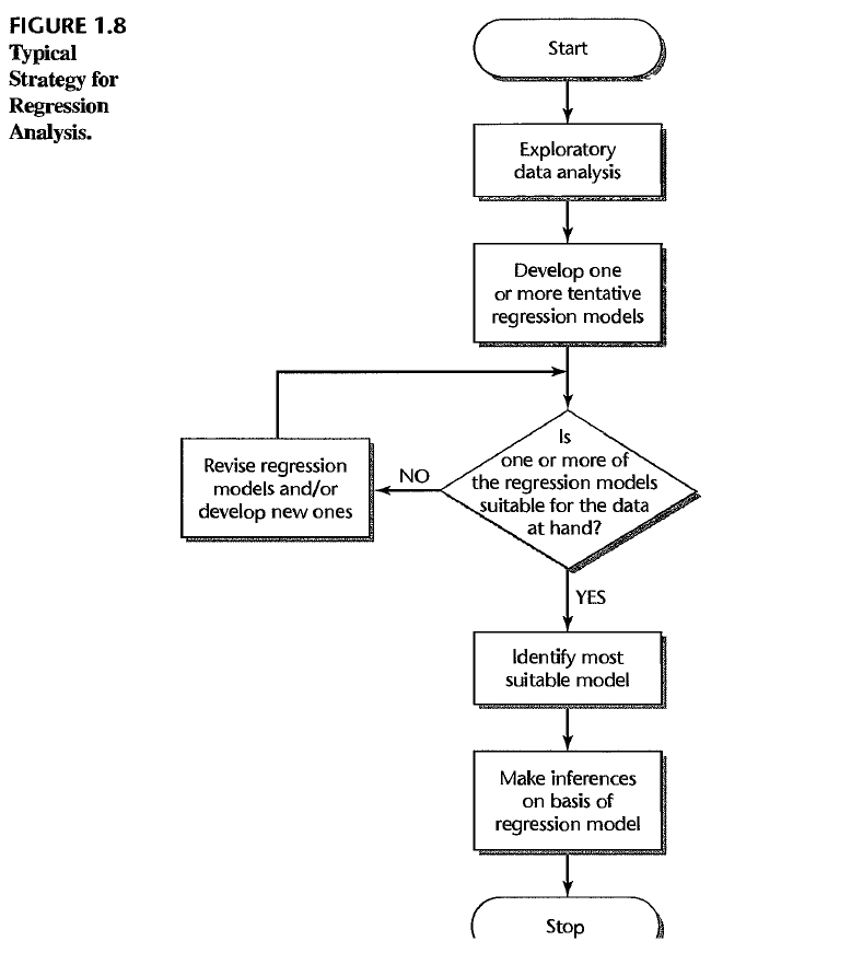
1.5 Overview of Steps in Regression Analysis

1.6 Estimation of Regression Function

1.6.1 Method of Least Squares

We are aiming to make $Y_i$ and $\beta_0+\beta_1 X_i$ close for all $i$, here we use Least Squares Estimation, which is

$$Q(b_0,b_1)=\min_{\beta_0,\beta_1}\sum_{i=1}^n\epsilon_i^2=\min_{\beta_0,\beta_1}\sum_{i=1}^n(Y_i-\beta_0-\beta_1 X_i)^2$$ $$SS_{XX}=\sum_{i=1}^n(X_i-\bar{X})^2=\sum_{i=1}^nX_i^2-n\bar{X}^2$$ $$SS_{YY}=\sum_{i=1}^n(Y_i-\bar{Y})^2=\sum_{i=1}^nY_i^2-n\bar{Y}^2$$ $$SS_{XY}=\sum_{i=1}^n(X_i-\bar{X})(Y_i-\bar{Y})=\sum_{i=1}^nX_iY_i-n\bar{X}\bar{Y}$$

Then find the least square estimators $b_0,b_1$ that minimize $Q$

$$\frac{\partial Q}{\partial\beta_0}=\frac{\partial Q}{\partial\beta_1}=0$$

Then we can find the estimators

$$b_1=\frac{SS_{XY}}{SS_{XX}},\quad b_0=\bar{Y}-b_1\bar{X}$$

True regression line is $Y=\beta_0+\beta_1X$, we have $\hat{Y}=b_0+b_1X$, and $E(b_0)=\beta_0,E(b_1)=\beta_1$

Residual: the difference between the observed and fitted predicted value. $e_i=Y_i-\hat{Y_i}=Y_i-(b_0+b_1X_i)$.

Model error: $\epsilon_i=Y_i-E(Y_i)=Y_i-(\beta_0+\beta_1X_i)$

Sum of Squared Residuals: $SSE=\sum_{i=1}^ne_i^2=\sum_{i=1}^n(Y_i-\hat{Y_i})^2$

The fitted values are calculated by

$$\hat{Y_i}=b_0+b_1X_i=(\bar{Y}-\frac{SS_{XY}}{SS_{XX}}\bar{X})+\frac{SS_{XY}}{SS_{XX}}X_i=\bar{Y}+\frac{SS_{XY}}{SS_{XX}}(X_i-\bar{X})$$

1.6.2 Properties of Fitted Regression Line

1. $\sum_{i=1}^ne_i=0$
2. $\sum_{i=1}^ne_i^2$ is minimized
3. $\sum_{i=1}^nY_i=\sum_{i=1}^n\hat{Y_i}$
4. $\sum_{i=1}^nX_ie_i=0$
5. $\sum_{i=1}^n\hat{Y_i}e_i=0$

Proof:

(1) $\sum_{i=1}^ne_i=\sum_{i=1}^n[Y_i-\bar{Y}-b_1(X_i-\bar{X})]=0\Rightarrow$ (3) $\sum_{i=1}^nY_i=\sum_{i=1}^n\hat{Y_i}$

(4) $\sum_{i=1}^nX_ie_i=\sum_{i=1}^n(X_i-\bar{X})e_i=\sum_{i=1}^n(X_i-\bar{X})[Y_i-\bar{Y}-b_1(X_i-\bar{X})]=SS_{XY}-b_1SS_{XX}=0$

(5) $\sum_{i=1}^n\hat{Y_i}e_i=\sum_{i=1}^ne_i[\bar{Y}+b_1(X_i-\bar{X})]=\bar{Y}\sum_{i=1}^ne_i+b_1\sum_{i=1}^ne_i(X_i-\bar{X})=0$

1.7 Estimation of Error Terms Variance $\sigma^2$

$$\sigma^2=Var(\epsilon)=E(\epsilon^2)$$

$\epsilon$ is unobservable, so we use residual $e$ to estimate $\epsilon$

$$s^2=\frac{1}{n-2}\sum_{i=1}^ne_i^2=\frac{1}{n-2}\sum_{i=1}^n(Y_i-\hat{Y_i})^2=\frac{SSE}{n-2}=MSE$$

Properties of Estimators:

Under linear regression model in which the errors have expectation zero and are uncorrelated and have equal variance $\sigma^2$.

1. Least squares estimators $b_0$ and $b_1$ are linear combinations of $\left\{Y_i\right\}$
2. (Gauss-Markov theorem) Least squares estimators $b_0$ and $b_1$ are BLUE (best linear unbiased estimators) of $\beta_0$ and $\beta_1$ respectively
3. MSE is an unbiased estimator of $\sigma^2$, i.e.$E(MSE)=\sigma^2$

Proof:

1- Linear combinations of $Y_i$

$$b_1=\frac{SS_{XY}}{SS_{XX}}=\frac{\sum_{i=1}^n(X_i-\bar{X})(Y_i-\bar{Y})}{SS_{XX}}=\sum_{i=1}^n\frac{(X_i-\bar{X})}{SS_{XX}}Y_i=\sum_{i=1}^nk_iY_i$$ $$b_0=\bar{Y}-b_1\bar{X}=\sum_{i=1}^n(\frac{1}{n}-k_i\bar{X})Y_i=\sum_{i=1}^nl_iY_i$$

here we have

$$k_i=\frac{X_i-\bar{X}}{SS_{XX}}$$ $$l_i=\frac{1}{n}-k_i\bar{X}$$

2- Best Linear Unbiased Estimator

Denote $k_i=\frac{X_i-\bar{X}}{SS_{XX}}$, note that $\sum_{i=1}^nk_i=0,\sum_{i=1}^nk_iX_i=1,\sum_{i=1}^nk_i^2=\frac{1}{SS_{XX}}$.

$E(b_1)=\sum_{i=1}^nk_iE(Y_i)=\sum_{i=1}^nk_i(\beta_0+\beta_1X_i)=\beta_0\sum_{i=1}^nk_i+\beta_1\sum_{i=1}^nk_iX_i=\beta_1$

$E(b_0)=E(\bar{Y}-b_1\bar{X})=(\beta_0+\beta_1\bar{X})-\beta_1\bar{X}=\beta_0$

So $b_0$ and $b_1$ are unbiased estimators of $\beta_0$ and $\beta_1$.

$var(b_1)=\sum_{i=1}^nk_i^2var(Y_i)=\sigma^2\sum_{i=1}^nk_i^2=\frac{\sigma^2}{SS_{XX}}$

$cov(b_1,Y_i)=cov(\sum_{i=1}^nk_iY_i,Y_i)=cov(k_iY_i,Y_i)=k_i\sigma^2$

$cov(b_1,\bar{Y})=cov(b_1,\sum_{i=1}^n\frac{1}{n}Y_i)=\frac{1}{n}\sum_{i=1}^nk_i\sigma^2=0$

$var(b_0)=var(\bar{Y}-b_1\bar{X})=var(\bar{Y})+\bar{X}^2var(b_1)-2\bar{X}cov(\bar{Y},b_1)=\sigma^2(\frac{1}{n}+\frac{\bar{X}^2}{SS_{XX}})$

$cov(b_0,b_1)=cov(\bar{Y}-b_1\bar{X},b_1)=-\bar{X}var(b_1)=-\frac{\bar{X}}{SS_{XX}}\sigma^2$

The variance matirx of $(b_0,b_1)$ is

$$\frac{\sigma^2}{SS_{XX}}\left(\begin{matrix} \frac{1}{n}\sum_{i=1}^nX_i^2 & -\bar{X}\\ -\bar{X} & 1 \end{matrix}\right)$$

Among all unbiased linear estimators of the form $\hat{\beta_1}=\sum c_iY_i$

$$\begin{aligned} E(\hat{\beta_1}) &=\sum c_iE(Y_i)=\sum c_i(\beta_0+\beta_1X_i)\\ &=\beta_0\sum c_i+\beta_1\sum c_iX_i=\beta_1 \end{aligned}$$

so that it must be the case that $\sum c_i=0$ and $\sum c_iX_i=1$.

Define $d_i=c_i-k_i$, where $k_i=\frac{X_i-\bar{X}}{SS_{XX}}$

$$\begin{aligned} var(\hat{\beta_1}) &= \sum c_i^2var(Y_i)=\sigma^2\sum(k_i+d_i)^2\\ &= \sigma^2(\sum k_i^2+\sum d_i^2 +2\sum k_id_i) \end{aligned}$$

Now by showing that

$$\begin{aligned} \sum k_id_i &= \sum k_i(c_i-k_i)=\sum k_ic_i-\sum k_i^2\\ &= \sum c_i(\frac{X_i-\bar{X}}{SS_{XX}})-\frac{1}{SS_{XX}}\\ &=\frac{\sum c_iX_i-\bar{X}\sum c_i-1}{SS_{XX}}=0 \end{aligned}$$

So that

$$var(\hat{\beta_1})=var(b_1)+\sigma^2(\sum d_i^2)$$

when $d_i=0$, the variance is minimized.

#TODO:Similarly, we can show $b_0$ is BLUE of $\beta_0$.

3- $E(MSE)=\sigma^2$

$e_i=Y_i-\hat{Y_i}=(Y_i-\bar{Y})-b_1(X_i-\bar{X})$

$E(e_i)=E(Y_i-b_0-b_1X_i)=\beta_0+\beta_1X_i-\beta_0-\beta_1X_i=0$

$$\begin{aligned} var(e_i)&=var[Y_i-\bar{Y}-b_1(X_i-\bar{X})]\\ &= var(Y_i)+var(\bar{Y})+(X_i-\bar{X})^2var(b_1)-2cov(Y_i,\bar{Y})\\ &\quad-2(X_i-\bar{X})[cov(Y_i,b_1)-cov(\bar{Y},b_1)]\\ &=\sigma^2+\frac{\sigma^2}{n}+\frac{(X_i-\bar{X})^2\sigma^2}{SS_{XX}}-\frac{2\sigma^2}{n}-\frac{2(X_i-\bar{X})^2\sigma^2}{SS_{XX}}\\ &=\frac{(n-1)\sigma^2}{n}-\frac{(X_i-\bar{X})^2\sigma^2}{SS_{XX}} \end{aligned}$$

$E(SSE)=\sum_{i=1}^nE(e_i^2)=\sum_{i=1}^nvar(e_i)=(n-1)\sigma^2-\sigma^2=(n-2)\sigma^2$

$E(MSE)=\frac{E(SSE)}{n-2}=\sigma^2$

Note: For any $i\not ={j}$, $\epsilon_i$ and $\epsilon_j$ are uncorrelated, but $e_i$ and $e_j$ are correlated.

$$\begin{aligned} 0 &= var(\sum_{i=1}^ne_i)=\sum_{i=1}^nvar(e_i)+\sum_{i,j=1,j\not ={i}}^n cov(e_i,e_j)\\ &\Rightarrow \sum_{i,j=1,j\not ={i}}^n cov(e_i,e_j)=-\sum_{i=1}^n var(e_i)=-(n-2)\sigma^2 \end{aligned}$$

It can be proved that

$$cov(e_i,e_j)=-\frac{\sigma^2}{n}-\frac{(X_i-\bar{X})(X_j-\bar{X})\sigma^2}{SS_{XX}}$$ $$0=[\sum_{i=1}^n(X_i-\bar{X})]^2=SS_{XX}+\sum_{i,j=1,j\not ={i}}^n(X_i-\bar{X})(X_j-\bar{X})$$

So that

$$\sum_{i,j=1,j\not ={i}}^n cov(e_i,e_j)=-(n-1)\sigma^2+\sigma^2=-(n-2)\sigma^2$$

1.8 Normal Error Regression Model

1.8.1 Method of Least Sqaures

$$Y_i=\beta_0+\beta_1X_i+\epsilon_i,i=1,2,...,n$$

where $\epsilon_i$ are i.i.d and $\epsilon_i\sim N(0,\sigma^2)$, so that $Y_i\sim N(\beta_0+\beta_1X_i,\sigma^2)$ and $\left\{Y_i\right\}$ are independent

$$f(y_i)=\frac{1}{\sqrt{2\pi\sigma^2}}\exp\left\{-\frac{(y_i-(\beta_0+\beta_1X_i))^2}{2\sigma^2}\right\}$$

Likelihood:

$$L(\beta_0,\beta_1,\sigma^2)=\prod_{i=1}^nf(y_i)=(2\pi\sigma^2)^{-n/2}\exp\left\{-\frac{1}{2\sigma^2}\sum_{i=1}^n(y_i-(\beta_0+\beta_1X_i))^2\right\}$$

Use method of least square to find the Maximum Likelihood Estimators (MLEs):

$$(\hat{\beta_0},\hat{\beta_1})=\argmax_{\beta_0,\beta_1}(\ln L)=\argmin_{\beta_0,\beta_1}\sum_{i=1}^n[y_i-(\beta_0+\beta_1X_i)]^2=(b_0,b_1)$$

then the MLEs are

$$\hat{\beta_1}=b_1=\frac{SS_{XY}}{SS_{XX}}$$ $$\hat{\beta_0}=b_0=\bar{Y}-\hat{\beta_1}\bar{X}$$ $$\hat{\sigma}^2=\frac{1}{n}\sum(Y_i-\bar{Y_i})^2=\frac{SSE}{n}=\frac{n-2}{n}MSE$$

1.8.2 Properties of MLEs

1- MLEs of $\beta_0$ and $\beta_1$ are same with LSE estimators $b_0$ and $b_1$. They are linear combinations of $\left\{Y_i\right\}$

2- MLEs of $\beta_0$ and $\beta_1$ are BLUEs and normal distributed

$$\left(\begin{matrix} \hat{\beta_0}\\\hat{\beta_1} \end{matrix}\right) \sim N\left(\left( \begin{matrix} \beta_0\\\beta_1 \end{matrix}\right), \frac{\sigma^2}{SS_{XX}} \left(\begin{matrix} \frac{1}{n}\sum X_i^2 & -\bar{X}\\ -\bar{X} & 1 \end{matrix}\right)\right)$$

3- MLE of $\sigma^2$ is a biased estimator with

$$\frac{n\hat{\sigma}^2}{\sigma^2}=\frac{SSE}{\sigma^2}\sim\chi^2(n-2)\quad\text{and}\quad E(\hat{\sigma}^2)=\frac{n-2}{n}\sigma^2\rightarrow\sigma^2$$

3- $(\hat{\beta_0},\hat{\beta_1},\bar{Y})$ and $\sigma^2$ are independent.

Proof:

4- This can be derived by Fisher’s theorem

$$\mu_i=E(Y_i)=\beta_0+\beta_1X_i=\beta_0^*+\beta_1(X_i-\bar{X}),\beta_0^*=\beta_0+\beta_1\bar{X}$$ $$\hat{\beta_0^*}=\bar{Y}\sim N(\beta_0^*,\sigma^2/n),\hat{\beta_1}=\frac{SS_{XY}}{SS_{XX}}\sim N(\beta_1,\sigma^2/SS_{XX})$$

then we have

$$\begin{aligned} \sum(Y_i-\mu_i)^2 &=\sum(\hat{Y_i}-\mu_i)^2+\sum(Y_i-\hat{Y_i})^2\\ &= \sum[\hat{\beta_0^*}+\hat{\beta_1}(X_i-\bar{X})-\beta_0^*-\beta_1(X_i-\bar{X})]^2+SSE\\ &= n(\hat{\beta_0^*}-\beta_0^*)^2+(\hat{\beta_1}-\beta_1)^2SS_{XX}+n\hat{\sigma}^2\\ \end{aligned}$$

With the Fisher’s theorem

$$Q/\sigma^2=Q_1/\sigma^2+Q_2/\sigma^2+Q_3/\sigma^2$$ $$\chi^2_n=\chi^2_1+\chi^2_1+\chi^2_{n-2}$$

Chap2 Inference in Regression and Correlation Analysis

Outline:

• Inferences Concerning $\beta_1,\beta_0$ and $EY$ in Normal Error Regression Model
• Prediction Interval of New Observation
• Confidence Band for Regression Line
• Analysis of Variance (ANOVA) approach to Regression Analysis
• General linear test approach
• Normal Correlation Models and Inferences

2.1 Inferences Concerning $\beta_1$

$$Y_i=\beta_0+\beta_1X_i+\epsilon_i,i=1,2,...,n$$

with $\epsilon_i$ are i.i.d and $\epsilon_i\sim N(0,\sigma^2)$.

$$b_1\sim N(\beta_1,\frac{\sigma^2}{SS_{XX}})\Rightarrow \frac{b_1-\beta_1}{\sqrt{\sigma^2/SS_{XX}}}=\frac{b_1-\beta_1}{\sigma\left\{b_1\right\}}\sim N(0,1)$$

since

$$\frac{(n-2)MSE}{\sigma^2}\sim\chi^2_{n-2},\quad b_1\perp MSE$$ $$\Rightarrow\frac{(b_1-\beta_1)/\sqrt{\sigma^2/SS_{XX}}}{\sqrt{\frac{(n-2)MSE}{\sigma^2}}/(n-2)}=\frac{b_1-\beta_1}{\sqrt{MSE/SS_{XX}}}=\frac{b_1-\beta_1}{s\left\{b_1\right\}}\sim t_{n-2}$$

where $\sigma\left\{b_1\right\}=\sqrt{\sigma^2/SS_{XX}},s\left\{b_1\right\}=\sqrt{MSE/SS_{XX}}$

2.2 Inferences Concerning $\beta_0$

$$b_0=\bar{Y}-b_1\bar{X}\sim N\left(\beta_0,\sigma^2\frac{\sum X_i^2}{nSS_{XX}}\right)=N\left(\beta_0,\sigma^2(\frac{1}{n}+\frac{\bar{X}^2}{SS_{XX}})\right)$$

since

$$\frac{(n-2)MSE}{\sigma^2}\sim\chi^2_{n-2},\quad b_0\perp MSE$$ $$\Rightarrow\frac{(b_0-\beta_0)/\sqrt{\sigma^2(\frac{1}{n}+\frac{\bar{X}^2}{SS_{XX}})}}{\sqrt{\frac{(n-2)MSE}{\sigma^2}/(n-2)}}=\frac{b_0-\beta_0}{\sqrt{MSE(\frac{1}{n}+\frac{\bar{X}^2}{SS_{XX}})}}=\frac{b_0-\beta_0}{s\left\{b_0\right\}}\sim t_{n-2}$$

where $\sigma\left\{b_0\right\}=\sqrt{\sigma^2(\frac{1}{n}+\frac{\bar{X}^2}{SS_{XX}})},s\left\{b_1\right\}=\sqrt{MSE(\frac{1}{n}+\frac{\bar{X}^2}{SS_{XX}})}$

2.3 Some Considerations on Making Inferences

• Effects of departures from normality of the $Y_i$
• Spacing of the $X$ levels
• Power of Tests

2.4 Interval Estimaton of $E\left\{Y_h\right\}$

Intersted in estimating the mean response for particular $X_h$

$$E\left\{Y_h\right\}=\beta_0+\beta_1X_h$$

The unbiased point estimator of $E\left\{Y_h\right\}$

$\hat{Y_h}=b_0+b_1X_h=\bar{Y}+b_1(X_h-\bar{X})$

$E(\hat{Y_h})=\beta_0+\beta_1X_h=E(Y_h)$

$var(\hat{Y_h})=var(\bar{Y})+(X_h-\bar{X})^2var(b_1)=\sigma^2(\frac{1}{n}+\frac{(X_h-\bar{X})^2}{SS_{XX}})$

So we have

$$\hat{Y_h}=\bar{Y}+b_1(X_h-\bar{X})\sim N\left(\beta_0+\beta_1X_h,\sigma^2[\frac{1}{n}+\frac{(X_h-\bar{X})^2}{SS_{XX}}]\right)$$

since

$$\frac{(n-2)MSE}{\sigma^2}\sim\chi^2_{n-2},\quad (b_0,b_1,\hat{Y_h})\perp MSE$$ $$\Rightarrow \frac{(\hat{Y_h}-E(Y_h))/\sqrt{\sigma^2(\frac{1}{n}+\frac{(X_h-\bar{X})^2}{SS_{XX}})}}{\sqrt{\frac{(n-2)MSE}{\sigma^2}/(n-2)}}=\frac{\hat{Y_h}-E(Y_h)}{\sqrt{MSE(\frac{1}{n}+\frac{(X_h-\bar{X})^2}{SS_{XX}})}}=\frac{\hat{Y_h}-E(Y_h)}{s\left\{\hat{Y_h}\right\}}\sim t_{n-2}$$

where $s\left\{\hat{Y_h}\right\}=\sqrt{MSE(\frac{1}{n}+\frac{(X_h-\bar{X})^2}{SS_{XX}})}$

2.5 Prediction of New Observation

Intersted in predicting new observation when $X=X_h$

$$Y_{hn}=\beta_0+\beta_1X_h+\epsilon_{hn}$$

here $Y_{hn}\perp\left\{Y_1,…,Y_n\right\}$ and

$$Y_{hn}\sim N(\beta_0+\beta_1X_h,\sigma^2)$$

Prediction of $Y_{hn}$

$$\hat{Y_h}=b_0+b_1X_h\sim N\left(\beta_0+\beta_1X_h,\sigma^2[\frac{1}{n}+\frac{(X_h-\bar{X})^2}{SS_{XX}}]\right)$$

Prediction error

$$Y_{hn}-\hat{Y_h}\sim N\left(0,\sigma^2[1+\frac{1}{n}+\frac{(X_h-\bar{X})^2}{SS_{XX}}]\right)$$

since

$$\frac{(n-2)MSE}{\sigma^2}\sim\chi^2_{n-2},\quad (Y_{hn},\hat{Y_h})\perp MSE$$ $$\Rightarrow \frac{Y_{hn}-\hat{Y_h}}{\sqrt{MSE(1+\frac{1}{n}+\frac{(X_h-\bar{X})^2}{SS_{XX}})}}=\frac{Y_{hn}-\hat{Y_h}}{s\left\{Y_{hn}-\hat{Y_h}\right\}}=\frac{Y_{hn}-\hat{Y_h}}{s\left\{pred\right\}}\sim t_{n-2}$$

where $s\left\{pred\right\}=\sqrt{MSE(1+\frac{1}{n}+\frac{(X_h-\bar{X})^2}{SS_{XX}})}=\sqrt{MSE+s^2\left\{\hat{Y_h}\right\}}$

2.6 Confidence Band for Regression Line

The $(1-\alpha)\times100\%$ Confidence interval of $E(Y_h)=\beta_0+\beta_1X_h$

$$s\left\{\hat{Y_h}\right\}=\sqrt{MSE(\frac{1}{n}+\frac{(X_h-\bar{X})^2}{SS_{XX}})}$$

The Working-Hotelling Confidence Band

Replace $t(1-\alpha/2,n-2)$ with Working-Hotelling value $W$ in each confidence interval

$$W=\sqrt{2F(1-\alpha;2,n-2)}\Rightarrow\hat{Y_h}\pm W\times s\left\{\hat{Y_h}\right\}$$

#TODO: It can be proved that

$$\max_{x_h}\left(\frac{\hat{Y_h}-E(Y_h)}{s\left\{\hat{Y_h}\right\}}\right)^2=\frac{(\bar{Y}-E\bar{Y})^2}{MSE/n}+\frac{(\hat{\beta_1}-\beta_1)^2}{MSE/SS_{XX}}$$ $$\frac{1}{2}\max_{x_h}\left(\frac{\hat{Y_h}-E(Y_h)}{s\left\{\hat{Y_h}\right\}}\right)^2\sim F(2,n-2)$$

2.7 ANOVA Approach to Regression

$$Y_i-\bar{Y}=(Y_i-\hat{Y_i})+(\hat{Y_i}-\bar{Y})$$

ANOVA: Analysis of Variance, it can be described with the deviation of observation $Y_i$ around the fitted line (i.e.$Y_i-\hat{Y_i}$) and the deviation of fitted value $\hat{Y_i}$ around the mean (i.e.$\hat{Y_i}-\bar{Y}$).

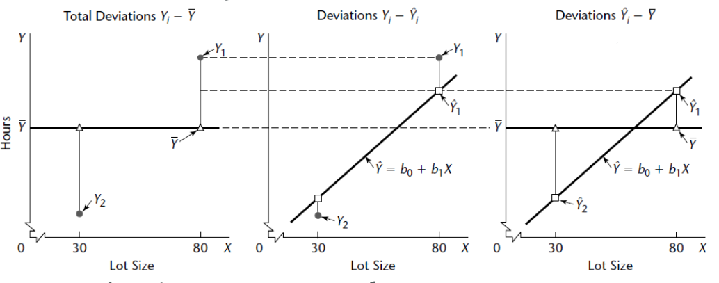
2.7.1 Partitioning of Total Sum of Squares

$$\sum_{i=1}^n(Y_i-\bar{Y})^2=\sum_{i=1}^n(\hat{Y_i}-\bar{Y})^2+\sum_{i=1}^n(Y_i-\hat{Y_i})^2+2\sum_{i=1}^n(Y_i-\hat{Y_i})(\hat{Y_i}-\bar{Y})$$

Because we have

$$\sum_{i=1}^n(Y_i-\hat{Y_i})(\hat{Y_i}-\bar{Y})=\sum_{i=1}^ne_i(\hat{Y_i}-\bar{Y})=\sum_{i=1}^ne_i\hat{Y_i}-\bar{Y}\sum_{i=1}^ne_i=0$$

then

$$\sum_{i=1}^n(Y_i-\bar{Y})^2=\sum_{i=1}^n(\hat{Y_i}-\bar{Y})^2+\sum_{i=1}^n(Y_i-\hat{Y_i})^2\\$$

SSTO: The total sum of squares

$$SSTO=\sum_{i=1}^n(Y_i-\bar{Y})^2$$

SSR: The sum squares explained by regression

$$SSR=\sum_{i=1}^n(\hat{Y_i}-\bar{Y})^2=b_1^2SS_{XX}$$

SSE: The sum squares explained by residual

$$SSE=\sum_{i=1}^n(Y_i-\hat{Y_i})^2$$ $$SSTO=SSR+SSE$$

In normal error regression model, we have

$$b_1\sim N(\beta_1,\frac{\sigma^2}{SS_{XX}})\Rightarrow \frac{b_1-\beta_1}{\sqrt{\sigma^2/SS_{XX}}}\sim N(0,1)$$ $$(b_0,b_1,\bar{Y})\perp SSE\Rightarrow SSR\perp SSE$$

Under $H_0:\beta_1=0$

$$\frac{SSE}{\sigma^2}=\frac{(n-2)MSE}{\sigma^2}\sim\chi^2_{n-2},\quad \frac{SSTO}{\sigma^2}\sim\chi_{n-1}^2$$ $$\frac{SSR}{\sigma^2}=\frac{b_1^2SS_{XX}}{\sigma^2}=\left(\frac{b_1-0}{\sqrt{\sigma^2/SS_{XX}}}\right)^2\sim\chi^2_1$$

Generally,

1- $\dfrac{SSE}{\sigma^2}\sim\chi^2_{n-2,0}$

2- $\dfrac{SSR}{\sigma^2}=\dfrac{b_1^2}{\sigma^2/SS_{XX}}\sim\chi^2_{1,\delta}$, where $\delta=\dfrac{\beta_1^2}{\sigma^2/SS_{XX}}$, since $b_1\sim N\left(\beta_1,\frac{\sigma^2}{SS_{XX}}\right)$

3- $SSR\perp SSE$

So that $\dfrac{SSTO}{\sigma^2}\sim\chi^2_{n-1,\delta}$

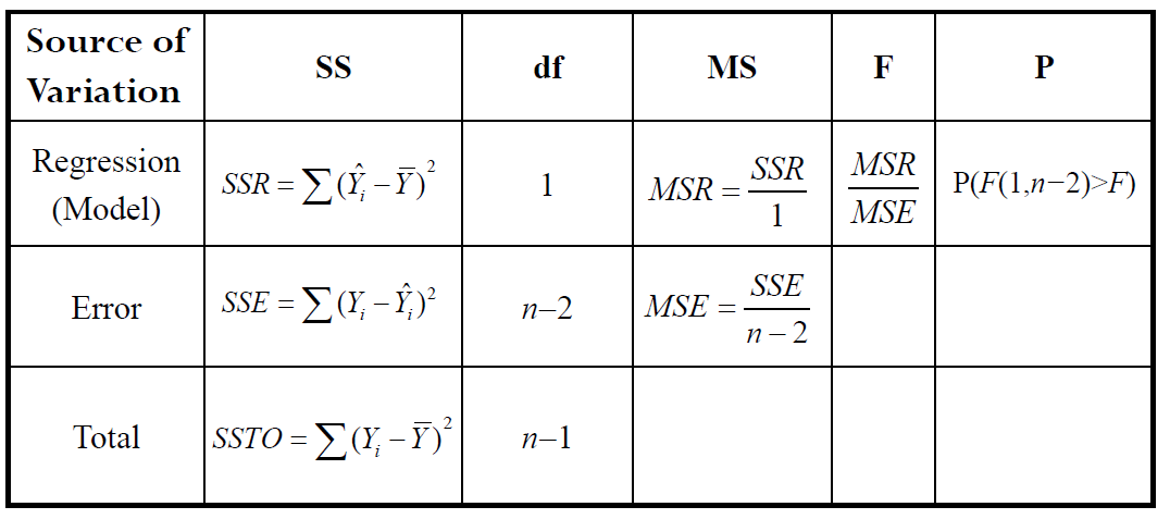
2.7.2 Mean Squares

$$MSR=SSR/1$$

$E(MSR)=E(SSR)=E(b_1^2SS_{XX})=SS_{XX}(\frac{\sigma^2}{SS_{XX}}+\beta_1^2)=\sigma^2+\beta_1^2SS_{XX}$

$$MSE=\frac{SSE}{n-2}$$

$E(MSE)=\sigma^2$

$$F^*=\frac{SSR/1}{SSE/(n-2)}=\frac{MSR}{MSE}\sim F_{1,n-2,\delta=\beta_1^2SS_{XX}/\sigma^2}$$

2.7.3 F test

Hypothesis: $H_0:\beta_1=0\quad v.s.\quad H_1:\beta_1\not ={0}$

$$F^*=\frac{MSR}{MSE}\stackrel{H_0}{\sim}F_{1,n-2}$$

When $H_0$ is false, $MSR>MSE$. Reject $H_0$ when $F^*$ large.

2.7.4 Equivalence of F test and two-sided t-test

Hypothesis: $H_0:\beta_1=0\quad v.s.\quad H_1:\beta_1\not ={0}$

$$F^*=\frac{MSR}{MSE}=\frac{b_1^2SS_{XX}}{MSE}=\left(\frac{b_1}{\sqrt{MSE/SS_{XX}}}\right)^2=(\frac{b_1}{s(b_1)})^2=(t^*)^2$$

In addition:

$$t^2_{n-2}\sim F_{1,n-2}\Rightarrow t^2_{1-\alpha/2;n-2}=F_{1-\alpha;1,n-2}$$

Equivalence of rejection regions:

$$F^*>F_{1-\alpha;1,n-2}\Leftrightarrow |t^*|>t^2_{1-\alpha/2;n-2}$$

2.8 General Linear Test Approach

Full/unrestricted model: $Y_i=\beta_0+\beta_1X_i+\epsilon_i$

Reduced/restricted model: $Y_i=\beta_0+\epsilon_i\quad Y_i\sim N(\beta_0,\sigma^2)$

Intuition: Compare the SSE’s of the two models to find out which model fits better. If SSE(F) not much smaller than SSE(R), full model doesn’t better explain Y.

Hypothesis: $H_0:\text{Reduced model}\quad v.s.\quad H_1:\text{Full model}$

Test statistic:

$$F^*=\frac{(SSE(R)-SSE(F))/(df_R-df_F)}{SSE(F)/df_F}\stackrel{H_0}{\sim}F_{df_R-df_F,df_F}$$

since $SSE(R)=(SSE(R)-SSE(F))+SSE(F)$, the degree of freedom can be calculate with Fisher’s Theorem.

Note: General linear test is equal to ANOVA test

$SSE(F)=SSE$

$SSE(R)=\sum(Y_i-\hat{Y_i}(R))^2=\sum(Y_i-\bar{Y})^2=SSTO,df_R=n-1$

$$F^*=\frac{(SSE(R)-SSE(F))/(df_R-df_F)}{SSE(F)/df_F}=\frac{(SSTO-SSE)/1}{SSE/(n-2)}=\frac{MSR}{MSE}$$

2.9 Descriptive Measures of Linear Association

Coefficient of Determination:

$$R^2=\frac{SSR}{SSTO}$$

which is the proportion of total variation $Y$ explained by $X$

Pearson’s Correlation Coefficient:

$$\rho=corr(X,Y)=\frac{cov(X,Y)}{\sqrt{var(X)var(Y)}}$$

which measures the strength of the linear relationship between two variables

$\rho$ can be estimated by

$$r=\frac{\frac{1}{n}\sum_{i=1}^n(X_i-\bar{X})(Y_i-\bar{Y})}{\sqrt{\frac{1}{n}\sum_{i=1}^n(X_i-\bar{X})^2\frac{1}{n}\sum_{i=1}^n(Y_i-\bar{Y})^2}}=\frac{SS_{XY}}{\sqrt{SS_{XX}SS_{YY}}}$$

For simple linear regression

$$b_1=\frac{SS_{XY}}{SS_{XX}}\Rightarrow R^2=\frac{SSR}{SSTO}=\frac{b_1^2SS_{XX}}{SS_{YY}}=\frac{SS_{XY}^2}{SS_{XX}SS_{YY}}$$ $$r=\frac{SS_{XY}}{\sqrt{SS_{XX}SS_{YY}}}=\sqrt{\frac{SS_{XX}}{SS_{YY}}}b_1=\frac{S_X}{S_Y}b_1$$

2.11 Normal correlation model

Note: In normal error regression model, we assume that the X values are known constants. A correlation model, takes each variable as random.

2.11.1 Bivariate Normal Distribution

The normal correlation model for the case of two variables is based on the bivariate normal distribution $N(\mu_1,\mu_2,\sigma^2_1,\sigma^2_2,\rho)$.

Density function:

$$f(Y_1,Y_2)=\frac{1}{2\pi\sigma_1\sigma_2\sqrt{1-\rho_{12}^2}}\exp \left\{-\frac{1}{2(1-\rho_{12}^2)}[(\frac{y_1-\mu_1}{\sigma_1})^2-2\rho_{12}(\frac{y_1-\mu_1}{\sigma_1})(\frac{y_2-\mu_2}{\sigma_2})+(\frac{y_2-\mu_2}{\sigma_2})^2]\right\}$$

Marginal Distribution:$Y_1\sim N(\mu_1,\sigma_1^2), Y_2\sim N(\mu_2,\sigma_2^2)$

Conditional Probability:

$$(Y_1|Y_2=y_2)\sim N(\mu_1+\rho_{12}\frac{\sigma_1}{\sigma_2}(y_2-\mu_2),\sigma_1^2(1-\rho_{12}^2))$$

2.11.2 Inference on $\rho_{12}$

Under bivariate normal assumption, the MLE of $\rho_{12}$

$$\hat{\rho_{12}}=r_{12}=\frac{SS_{XY}}{\sqrt{SS_{XX}SS_{YY}}}$$

Interst in testing $H_0:\rho_{12}=0 \Leftrightarrow\beta_{12}=\beta_{21}=0$

$$\frac{r_{12}}{\sqrt{(1-r_{12}^2)/(n-2)}}=\frac{\frac{S_X}{S_Y}b_1}{\sqrt{\frac{SSE}{SSTO}/(n-2)}}=\frac{b_1}{\sqrt{MSE/SS_{XX}}}=\frac{b_1}{s(b_1)}\stackrel{H_0}{\sim}t_{n-2}$$

Test statistic:

$$t^*=\frac{r_{12}\sqrt{n-2}}{\sqrt{1-r_{12}^2}}$$

Interval Estimation: (when $\rho_{12}\not ={0}$)

$$z'=\frac{1}{2}\ln(\frac{1+r_{12}}{1-r_{12}})\stackrel{approx}{\sim}N(\zeta,\frac{1}{n-3})$$ $$\zeta=\frac{1}{2}\ln(\frac{1+\rho_{12}}{1-\rho_{12}})$$

CI for $\zeta=z’\pm z_{1-\alpha/2}\sqrt{\frac{1}{n-3}}=(c_1,c_2)$

CI for $\rho_{12}=(\frac{e^{2c_1}-1}{e^{2c_1}+1},\frac{e^{2c_2}-1}{e^{2c_2}+1})$

2.11.3 Spearman’s correlation method

Rank $(Y_{11},…,Y_{n1})$ from 1 to n and label:$(R_{11},…,R_{n1})$, rank $(Y_{12},…,Y_{n2})$ from 1 to n and label:$(R_{12},…,R_{n2})$.

$$r_s=\frac{\sum_{i=1}^n(R_{i1}-\bar{R_1})(R_{i2}-\bar{R_2})}{\sqrt{\sum_{i=1}^n(R_{i1}-\bar{R_1})^2\sum_{i=1}^n(R_{i2}-\bar{R_2})^2}}$$

Hypothesis: $H_0$: No Association Between $Y_1,Y_2\quad$v.s.$\quad H_A$: Association Exists

Test Statistic(when there is no tie):

$$t^*=\frac{r_s\sqrt{n-2}}{\sqrt{1-r_s^2}}\stackrel{H_0}{\sim}t(n-2)$$

Chap3 Diagnostics and Remedial Measures

Outline:

• Diagnostics for prediction variable
• Diagnostics for residuals
• Remedial Measures

3.1 Diagnostics for prediction variable

• Scatterplot
• Dot plot or bar plot
• Histogram or stem-and-leaf plot
• Box plot
• Sequence plot

3.2 Residuals

In a normal regression model we assume that

$$\epsilon_i=Y_i-E(Y_i)=Y_i-(\beta_0+\beta_1X_i)\stackrel{i.i.d}{\sim}N(0,\sigma^2)$$

And we define residuals as

$$e_i=Y_i-\hat{Y_i}=Y_i-(b_0+b_1X_i)=Y_i-\bar{Y}-b_1(X_i-\bar{X})$$

The properties of the residuals:

1. $\sum_{i=1}^ne_i=\sum_{i=1}^nX_ie_i=\sum_{i=1}^n\hat{Y_i}e_i=0$
2. $e_i$ are normal distributed but not independent. When n large, the dependency can be ignored.

Proof:

$e_i=Y_i-\hat{Y_i}\sim N(0,(1-h_{ii})\sigma^2),\quad cov(e_i,e_j)=-h_{ij}\sigma^2\not ={0},i\not ={j}$

where $h_{ij}=\frac{1}{n}+\frac{(X_i-\bar{X})(X_j-\bar{X})}{SS_{XX}}$

$\begin{aligned}var(e_i)&=var(Y_i)+var(\bar{Y})+var(b_1)(X_i-\bar{X})^2-2cov(Y_i,\bar{Y})-2(X_i-\bar{X})cov(Y_i,b_1)\\&=\sigma^2+\frac{\sigma^2}{n}+\frac{(X_i-\bar{X})^2\sigma^2}{SS_{XX}}-\frac{2\sigma^2}{n}-\frac{2(X_i-\bar{X})^2\sigma^2}{SS_{XX}}\\&=\sigma^2(1-\frac{1}{n}-\frac{(X_i-\bar{X})^2}{SS_{XX}})\end{aligned}$

Chap 5 Matrix Approach

5.1 Matrix properties

Trace: $tr(A)=\sum_i a_{ii}$

$$tr(A+B)=tr(A)+tr(B)，tr(A)=tr(A^T)，tr(AB)=tr(BA)$$

Idempotent: $A^2=A\Rightarrow A^n=A$

1. A idempotent matrix is always diagonalizable and its eigenvalues are either 0 or 1. $$\lambda x=Ax=A^2x=\lambda^2x\Rightarrow \lambda=0\text{ or }1$$
2. For an idempotent matrix, $rank(A)=tr(A)$ or the number of non-zero eigenvalues of $A$
3. For $A_1,A_2$ are idempotent matrices $$A_1+A_2 \text{ is idempotent }\Leftrightarrow A_1A_2=A_2A_1=0\\ A_1-A_2 \text{ is idempotent }\Leftrightarrow A_1A_2=A_2A_1=A_2$$
4. $A$ is idempotent $\Rightarrow I-A$ is idempotent

5.2 Basic result

5.2.1 Variance-Covariance matrix

Suppose the random vector $Y$ consitsting of three observations.

$$\begin{aligned} var(Y)&=E\left\{[Y-E(Y)][Y-E(Y)]^T\right\}\\ &=\begin{bmatrix} \sigma^2_1&\sigma_{12}&\sigma_{13}\\ \sigma_{21}&\sigma^2_2&\sigma_{23}\\ \sigma_{31}&\sigma_{32}&\sigma^2_3 \end{bmatrix} \end{aligned}$$

5.2.2 Covariance matrix

Suppose the random vector $X$ consitsting of $m$ observations and $Y$ consisting of $n$ observations.

$$\begin{aligned} cov(X,Y)&=E\left\{[X-E(X)][Y-E(Y)]^T\right\}\\ &=\begin{bmatrix} \sigma_{11}&\cdots&\sigma_{1n}\\ \vdots&&\vdots\\ \sigma_{m1}&\cdots&\sigma_{mn}\\ \end{bmatrix} \end{aligned}$$

where $\sigma_{ij}=cov(X_i,Y_j)$

5.2.3 Expectation and variance

For constant matrices $A,B$ and random vector$Y$

$$E(AY)=AE(Y),var(AY)=Avar(Y)A^T\\ cov(AY,BY)=Avar(Y)B^T$$

If $E(Y)=\mu,var(Y)=\Sigma=(\sigma_{ij})$, then

$$E(Y^TAY)=\mu^TA\mu+tr(A\Sigma)$$

Proof:

$$\quad E(Y^TAY)=\sum_{i,j}a_{ij}E(Y_iY_j)=\sum_{i,j}a_{ij}(\mu_j\mu_j+\sigma_{ij})=\mu^TA\mu+tr(A\Sigma)$$

5.2.4 Multivariate Normal Distribution

Multivariate Normal Density function of $Y\sim N(\mu,\Sigma)$:

$$f(Y)=(2\pi)^{-n/2}|\Sigma|^{-1/2}\exp[\frac{-1}{2}(Y-\mu)^T\Sigma^{-1}(Y-\mu)]$$

then $Y_i\sim N(\mu_i,\sigma^2_i),cov(Y_i,Y_j)=\sigma_{ij}$.

Note: if $A$ is a full rank constant matrix, then $AY\sim N(A\mu,A\Sigma A^T)$

5.3 Matrix Simple Linear Regression

$$Y_i=\beta_0+\beta_1X_i+\epsilon_i$$

Design matrix is defined as $n\times p$ matrix, with n observations and p variables

$$Y=\begin{bmatrix} Y_1\\Y_2\\\vdots\\Y_n \end{bmatrix}, X=\begin{bmatrix} 1&X_1\\ 1&X_2\\ \vdots&\vdots\\ 1&X_n\\ \end{bmatrix}, \beta=\begin{bmatrix} \beta_0\\\beta_1\\ \end{bmatrix}, \epsilon=\begin{bmatrix} \epsilon_1\\\epsilon_2\\\vdots\\\epsilon_n\\ \end{bmatrix}$$

then the Linear Regression Model can be written as $Y=X\beta+\epsilon$ and $Y\sim N(X\beta,\sigma^2I)$

1. $\epsilon\sim N(0,\sigma^2I)$
2. $E(Y)=X\beta +E(\epsilon)=X\beta$
3. $var(Y)=var(\epsilon)=\sigma^2I$

5.3.1 Some matrices properties

$$Y^TY=\sum_{i}Y_i^2, X^TX=\begin{bmatrix} n&\sum_i X_i\\ \sum_i X_i&\sum_i X_i^2\\ \end{bmatrix}, X^TY=\begin{bmatrix} \sum_i Y_i\\\sum_i X_iY_i \end{bmatrix}$$

Note: $\sum_i X_i^2=\sum_i(X_i-\bar{X})^2+n\bar{X}^2$, so that

$$|X^TX|=n\sum_i X_i^2-(\sum_i X_i)^2=nSS_{XX}$$ $$\begin{aligned} \Rightarrow (X^TX)^{-1}&=\frac{1}{nSS_{XX}} \begin{bmatrix} \sum_i X_i^2&-\sum_i X_i\\ -\sum_i X_i& n\\ \end{bmatrix}\\ &=\frac{1}{SS_{XX}} \begin{bmatrix} \frac{SS_{XX}}{n}+\bar{X}^2&-\bar{X}\\ -\bar{X}&1\\ \end{bmatrix} \end{aligned}$$

5.3.2 Estimating the parameters

Matrix derivation rules:

$$\frac{\partial A\beta}{\partial\beta}=A,\frac{\partial \beta^TA}{\partial\beta}=A^T,\frac{\partial\beta^TA\beta}{\partial\beta}=\beta^T(A+A^T)$$

L2-loss is defined as:

$$Q=(Y-X\beta)^T(Y-X\beta)=Y^TY-2Y^TX\beta+\beta^TX^TX\beta$$

Solve $\frac{\partial Q}{\partial \beta}=0$, which we obtain $X^TXb=X^TY\Rightarrow b=(X^TX)^{-1}X^TY$

$$E(b)=(X^TX)^{-1}X^TE(Y)=\beta$$ $$\begin{aligned} var(b)&=(X^TX)^{-1}X^Tvar(Y)[(X^TX)^{-1}X^T]^T\\ &=\sigma^2(X^TX)^{-1} \end{aligned}$$

so that $b\sim N(\beta,\sigma^2(X^TX)^{-1})$

5.3.3 Fitted value

$$\hat{Y}_i=b_0+b_1X_i\Rightarrow \hat{Y}=Xb=X(X^TX)^{-1}X^TY$$

Hat matirx:

$$H=X(X^TX)^{-1}X^T$$

where $h_{ij}=\frac{1}{n}+\frac{(X_i-\bar{X})(X_j-\bar{X})}{SS_{XX}}$.

Note: H is actually a projection matrix, which projects the observed value $Y$ onto the space that is spanned by the variables in $X$.

$$E(\hat{Y})=HE(Y)=HX\beta=X\beta,var(\hat{Y})=Hvar(Y)H^T=\sigma^2H$$ $$\hat{Y}=HY\sim N(X\beta,\sigma^2H)$$

5.3.4 Properties of hat matrix

1. Projection matrix: $HY=\hat{Y},HX=X,H\hat{Y}=\hat{Y},He=0$
2. Symmetric: $H^T=H$
3. Idempotent: $H^2=H$

5.3.5 Residuals

$$e_i=Y_i-\hat{Y}_i \Rightarrow e=Y-\hat{Y}=(I-H)Y$$

Note that the matrix $I-H$ is also symmetric and idempotent.

$$E(e)=(I-H)E(Y)=0$$ $$var(e)=(I-H)\sigma^2I(I-H)^T=\sigma^2(I-H)$$

so that $e\sim N(0,\sigma^2(I-H))$

5.3.6 Analysis of Variance

Note that $Y^TY=\sum Y_i^2,Y^TJY=(\sum_iY_i)^2$

$$SSTO=\sum(Y_i-\bar{Y})^2=\sum Y_i^2-\frac{1}{n}(\sum Y_i)^2$$ $$SSE=\sum(Y_i-\hat{Y}_i)^2=e^Te$$ $$SSR=SSTO-SSE$$

so that we have

$$SSTO=Y^T(I-\frac{1}{n}J)Y, rank(I-\frac{1}{n}J)=n-1$$ $$SSE=Y^T(I-H)Y,rank(I-H)=n-2$$ $$SSR=Y^T(H-\frac{1}{n}J)Y,rank(H-\frac{1}{n}J)=1$$

Note that $H,\frac{J}{n},I-\frac{J}{n},I-H,H-\frac{J}{n}$ are idempotent and symmetric

$$rank(H)=tr(X(X^TX)^{-1}X^T)=tr(I)=p$$

Quadratic forms for ANOVA:

$SSTO=Y^T(I-\frac{1}{n}J)Y\sim \sigma^2\chi^2(n-1,\delta)$

$SSE=Y^T(I-H)Y\sim\sigma^2\chi^2(n-2,0)$

$SSR=Y^T(H-\frac{1}{n}J)Y\sim\chi^2(1,\delta)$

where $\delta=\frac{1}{\sigma^2}(X\beta)^T(I-\frac{1}{n}J)X\beta=\frac{\beta_1^2}{\sigma^2/SS_{XX}}$

Cochran’s Theorem(Corollary): Let $X\sim N(\mu,\sigma^2I)$, A is symmetric with $rank(A)=r$, and $\delta=\mu^TA\mu/\sigma^2$ then

$$\frac{X^TAX}{\sigma^2}\sim\chi^2(r,\delta)\Leftrightarrow \text{A is idempotent}$$

Proof: there exists $A$ satisfies $A^TA=A^T(I-H)A=I_{n-p}$ ???

5.3.7 Inference in Regression Analysis

Parameters: use MSE to estimate $\sigma^2(b)$

$$s^2(b)=MSE(X^TX)^{-1}$$

Estimated mean response at $X=X_h$

$X_h=[1,X_h]$ then $\hat{Y}_h=X_hb$

$$s^2(\hat{Y}_h)=MSE(X_h(X^TX)^{-1}X_h^T)$$

Predicted new response at $X=X_h$

$$s^2(pred)=MSE(1+X_h(X^TX)^{-1}X_h^T)$$

Chap 6 Multiple Regression I

Outline:

• Multiple regression models
• General linear regression model in matrix form
• Inference about regression parameters
• Estimation of mean response and prediction
• Diagnostic and Remedial Measures

6.1 Multiple regression models

• Can include polynomial terms to deal with nonlinear realtions
• Can include product terms for interactions
• Can include dummy variables for categorical predictors

First-order model with 2 numeric predictors:

$$Y_i=\beta_0+\beta_1X_{i1}+\beta_2X_{i2}+\epsilon_i$$

here $X_1,X_2$ are additive and there is no interaction, $E(\epsilon_i)=0$

Interaction model:

$$Y=\beta_0+\beta_1X_1+\beta_2X_2+\beta_3X_1X_2+\epsilon$$

here the effect of $X_1$ depends on level of $X_2$

General linear regression model:

$$Y_i=\beta_0+\beta_1X_{i1}+\beta_2X_{i2}+...+\beta_{p-1}X_{i,p-1}+\epsilon_i$$

which defines a hyperplane in p-dimensions. Here we assumes the error terms have Normality, Independence and constant variance $\epsilon_i\sim NID(0,\sigma^2)$

Other special types: dummy variables, polynomial terms, transformed response variable etc.

6.2 General Linear Regression Model in Matrix Form

Design matrix: same as Chap5, a $n\times p$ matrix

$$Y= \begin{bmatrix} Y_1\\Y_2\\\vdots\\Y_n\\ \end{bmatrix}, X= \begin{bmatrix} 1 & X_{11} & \cdots & X_{1,p-1}\\ 1 & X_{21} & \cdots & X_{2,p-1}\\ \vdots & \vdots & & \vdots \\ 1 & X_{n1} & \cdots & X_{n,p-1}\\ \end{bmatrix}, \beta= \begin{bmatrix} \beta_0\\\beta_1\\\vdots\\\beta_{p-1}\\ \end{bmatrix}, \epsilon= \begin{bmatrix} \epsilon_1\\\epsilon_2\\\vdots\\\epsilon_n\\ \end{bmatrix}$$

then we write $Y=X\beta+\epsilon$ and $E(Y)=X\beta, \sigma^2(Y)=\sigma^2I$

6.3 Estimation of Regression Coefficients

Least Squares Estimation:

$$Q=(Y-X\beta)^T(Y-X\beta)$$

Solve the equation $\frac{\partial Q}{\partial \beta}=0$ to obtain the estimator

$$b=(X^TX)^{-1}X^TY$$

Maximum Likelihood Estimation:

$$L(\beta,\sigma^2)=(2\pi\sigma^2)^{-n/2}\exp[\frac{-1}{2\sigma^2}(Y-X\beta)^T(Y-X\beta)]$$

which leads to the same estimation as LSE since minimize $L(\beta,\sigma^2)$ are equivalent to minimize $Q$.

6.4 Fitted Values and Residuals

Hat matrix $H=X(X^TX)^{-1}X^T$ and fitted values $\hat{Y}=X\beta=HY\sim N(X\beta,\sigma^2H)$

Residuals $e=(I-H)Y\sim N(0,(I-H)\sigma^2)$

The properties of hat matrix is mentioned in Chap5.(Projection matrix, symmetric and idempotent, rank equals to p)

Denote that $H=(h_{ij})$, then

1. $h_{ii}=\sum_j h_{ij}^2$
2. $\sum_i h_{ii}=tr(H)=p$
3. $\sum_i h_{ij}=\sum_j h_{ij}=1$
4. $h_{ij}^2\leq h_{ii}h_{jj}$
5. $h_{ii}\geq \frac{1}{n}$

Proof:

1- $H=H^2\Rightarrow h_{ii}=\sum_j h_{ij}h_{ji}=\sum_j h_{ij}^2$

2- $\sum_i h_{ii}=tr(H)=tr(H^TH)=p$

3- $HX=X$, compare the first column then we have $\sum_j h_{ij}=1$, then due to the symmetry of $H$, $\sum_i h_{ij}=\sum_j h_{ij}=1$

4- $h_{ij}=X_i(X^TX)^{-1}X_j^T$, since $(X^TX)^{-1}$ is positive definite, define the inner product $=X_i(X^TX)^{-1}X_j^T$, with Cauchy-Schwarts inequality, $h_{ij}=|| \leq\sqrt{}=\sqrt{h_{ii}h_{jj}}$

5- Define $P=H-C$, where $C=\frac{1}{n}J$, then

$$P^2=H^2-HC-CH+C^2=H-HC-CH+C$$

$C$ is in the column space of $X$ since $span(1,…,1)\subset Col(X)$, $HC=C$. Also we know that $C=C(H+(I-H))$, $C(I-H)=0$ since $I-H$ projects onto $Col(X)^\perp$, then $C=CH$.

$P^2=H-C=P$ so $P$ is also a projection matrix, $h_{ii}=p_{ii}+c_{ii}=p_{ii}+\frac{1}{n}$ which means that $h_{ii}\geq\frac{1}{n}$

6.5 Analysis of Variance

Same as Chap5,

$$SSTO=Y^T(I-\frac{1}{n}J)Y, rank(I-\frac{1}{n}J)=n-1$$ $$SSE=Y^T(I-H)Y,rank(I-H)=n-p$$ $$SSR=Y^T(H-\frac{1}{n}J)Y,rank(H-\frac{1}{n}J)=p-1$$

Cochran’s Theorem(Ch6page25)

$$MSR=\frac{SSR}{p-1}=\frac{1}{p-1}Y^T(H-\frac{1}{n}J)Y$$ $$MSE=\frac{SSE}{n-p}=\frac{1}{n-p}Y^T(I-H)Y$$

here $E(MSR)\geq E(MSE)=\sigma^2$ and equal when all $\beta_i=0$

Hypothesis: $H_0:\beta_1=…=\beta_{p-1}=0\quad\text{v.s.}\quad H_1:\text{not all }\beta_i=0$

Test Statistic:

$$F^*=\frac{MSR}{MSE}=\frac{SSR/p-1}{SSE/n-p}\stackrel{H_0}{\sim}F(p-1,n-p)$$

Adjusted R square:

$$R_a^2=1-\frac{SSE/n-p}{SSTO/n-1}=1-\frac{MSE}{MSTO}$$

6.6 Inferences about Regression Parameters

6.6.1 Independence of b and SSE

$$e=(I-H)Y,b=(X^TX)^{-1}X^TY$$ $$\begin{aligned} cov(e,b)&=(I-H)\sigma^2(Y)[(X^TX)^{-1}X^TY]^T\\ &=\sigma^2(I-H)X(X^TX)^{-1}\\ &=0 \end{aligned}$$

6.6.2 Parameters estimators

Since $b=(X^TX)^{-1}X^TY\sim N(\beta,\sigma^2(X^TX)^{-1})$, the variance can be estimated by

$$s^2(b)=MSE(X^TX)^{-1}$$

Denote $A=(X^TX)^{-1}=(a_{ij})$, then $b_k\sim N(\beta_k,\sigma^2(b_k))$, with $\sigma^2(b_k)=a_{k+1,k+1}\sigma^2$, then the variance estimator is

$$s^2(b_k)=MSEa_{k+1,k+1}=SSEa_{k+1,k+1}/(n-p)$$

Since $b_k$ is independent with $SSE$,

$$\frac{b_k-\beta_k}{s(b_k)}=\frac{(b_k-\beta_k)/\sigma(b_k)}{\sqrt{\frac{SSE}{\sigma^2}/(n-p)}}\sim t(n-p)$$

then the CI for parameters can be constructed with

$$b_k\pm t(1-\frac{\alpha}{2};n-p)s(b_k)$$

the simultaneous CI’s for $g\leq p$

$$b_k\pm t(1-\frac{\alpha}{2g};n-p)s(b_k)$$

Hypothesis: $H_0:\beta_k=0\quad\text{v.s.}\quad H_1:\beta_k\neq 0$

Test Statistic:

$$t^*=\frac{b_k}{s(b_k)}\stackrel{H_0}{\sim}t(n-p)$$

6.7 Estimating mean response & New observations

6.7.1 Estimating mean response

Given set of levels of $X_1,…,X_{p-1}$

$$X_h=[1,X_{h1},...,X_{h,p-1}],\hat{Y_h}=X_hb$$ $$E(\hat{Y}_h)=X_h\beta,\sigma^2(\hat{Y}_h)=\sigma^2X_h(X^TX)^{-1}X_H^T$$

the variance can be estimated by $s^2(\hat{Y}_h)=MSE(X_h(X^TX)^{-1}X_h^T)=X_hs^2(b)X_h^T$.

Note: We denote $X_h$ as a row vector, notice the difference beween here and textbook

Similarly, we have $\hat{Y}_h\perp SSE$,

$$\frac{\hat{Y_h}-E(\hat{Y}_h)}{s(\hat{Y}_h)}=\frac{(\hat{Y}_h-E(\hat{Y}_h))/\sigma(\hat{Y}_h)}{\sqrt{\frac{SSE}{\sigma^2}/(n-p)}}\sim t(n-p)$$

CI for $E(\hat{Y}_h)$: $\hat{Y}_h\pm t(1-\frac{\alpha}{2};n-p)s(\hat{Y}_h)$

CI for g $E(\hat{Y}_h$: $\hat{Y}_h\pm B\cdot s(\hat{Y}_h)$

Confidence Region for Regression Surface: $\hat{Y}_h\pm W\cdot s(\hat{Y}_h)$

where $B=t(1-\frac{\alpha}{2g};n-p),W=\sqrt{pF(1-\alpha;p,n-p)}$

6.7.2 Prediction of New Observations

Predicted new response at $X_{new}=X_h$

$\hat{Y}_{h(new)}=X_hb\sim N(X_h\beta,\sigma^2X_h(X^TX)^{-1}X_h^T)$

Prediction error $Y_{h(new)}-\hat{Y}_{h(new)}\sim N(0,\sigma^2(1+X_h(X^TX)^{-1}X_h^T))$

the variance can be estimated by $s^2(pred)=MSE(1+X_h(X^TX)^{-1}X_h^T)$, such that

$$\frac{Y_{h(new)}-\hat{Y}_h}{s(pred)}\sim t(n-p)$$

The prediction interval of $Y_{h(new)}$ is

$$\hat{Y}_h\pm t(1-\frac{\alpha}{2};n-p)s(pred)$$

Bonferroni: prediction interval for g $Y_{h(new)}$ is

$$\hat{Y}_h\pm B\cdot s(pred),B=t(1-\frac{\alpha}{2g};n-p)$$

6.8 Diagnostics and Remedial Measures

The methods are similar to simple linear regression. Here are some other different methods:

6.8.1 Scatterplot matrix

Summarizes bivariate relationships between $Y$ and $X_j$ as well as between $X_j$ and $X_k$

6.8.2 Correlation Matrix

Displays all pairwise correlations

6.8.3 Residual Plots

Plot $e$ vs $\hat{Y},X_j$ and missing variable. This is used for similar assessment of assumptions: Linear, Independence, Normality, Equal variance, omitted variables, outliers

6.9 Tests for Diagnosis

• Correlation test for normality
• Brown-Forsythe Test for Constancy of Error variance
• Breusch-Pagan Test for Constancy of Error variance
• F-test for Lack of fit
• Box-Cox Transformations

6.9.1 Breusch-Pagan Test

Hypothesis: $H_0:\sigma^2(\epsilon_i)=\sigma^2\quad\text{v.s.}\quad H_1:\sigma^2(\epsilon_i)=\sigma^2h(\gamma_1X_{i1}+…+\gamma_kX_{ik})$

Denote $SSE=\sum_i e_i^2$ from original regression, fit reression of $e_i^2$ on $X_{i1},…,X_{ik}$ and obtain $SS(Reg^*)$

Test Statistic:

$$X_{BP}^2=\frac{SS(Reg^*)/2}{(\sum_i e_i^2/n)^2}\stackrel{H_0}{\sim}\chi_k^2$$

6.9.2 Lack of Fit Test

This method is available when there are replicates in some X levels. Define X levels as $X_1,…,X_c$ with $n_j$ replicates respectively and $\sum_j nj=n$.

(reduced) linear model

$H_0:E(Y_i)=\beta_0+\beta_1X_{i1}+…+\beta_{p-1}X_{i,p-1}$

(full) there are c parameters $\hat{\mu}_j=\bar{Y}_j$

$H_1:E(Y_i)\neq\beta_0+\beta_1X_{i1}+…+\beta_{p-1}X_{i,p-1}$

$$SSE=SSE(R)=\sum_j\sum_i(Y_{ij}-\hat{Y}_{ij})^2,df_R=n-p$$ $$SSPE=SSE(F)=\sum_j\sum_i(Y_{ij}-\bar{Y}_j)^2,df_F=n-c$$ $$SSLE=SSE-SSPE=\sum_jn_j(\bar{Y}_j-\hat{Y}_{ij})^2$$

Test Statistic:

$$F^*=\frac{SSLE/c-p}{SSPE/n-c}\sim F(c-p,n-c)$$

when $H_0$ is rejected, a more complex model is required.

Chap 7 Multiple Regression II

Outline:

• Extra Sums of Squares
• General Linear Test
• Partial Determination and Partion Correlation
• Standardized Version of the Multiple Regression Model
• Multicollinearity

7.1 Extra Sums of Squares

Basic Ideas: An extra sum of squares measures the marginal reduction in the error sum of squares when one or several predictor variables are added to the regression model, given that other predictor variables are already in the model.(or the increase in the regression sum of squares)

For a given dataset, the total sum of squares (SSTO) remains the same. As we include more predictors, the regression sum of squares (SSR) increases and the error sum of squares (SSE) decreases.

Define extra sum of squares:

$$\begin{aligned} SSR(X_2|X_1)&=SSR(X_1,X_2)-SSR(X_1)\\ &=SSE(X_1)-SSE(X_1,X_2) \end{aligned}$$

According to the Fisher’s Theorem:

$$SSR(X_1,X_2)=SSR(X_1)+SSR(X_2|X_1)$$ $$\sigma^2\chi^2(2,\delta_{R_2})=\sigma^2\chi^2(1,\delta_{R_1})+\sigma^2\chi^2(1,\delta_{R_2}-\delta_{R_1})$$

where $\delta_{R_1}=\frac{1}{\sigma^2}SS_{XX}\beta_1^2,\delta_{R_2}=\frac{1}{\sigma^2}\sum\sum SS_{kl}\beta_k\beta_l$

and $\delta_{R_2}-\delta_{R_1}=0$, if $\beta_2=0$

Decomposition of SSR:

$$SSR(X_1,X_2,X_3)=SSR(X_1)+SSR(X_2|X_1)+SSR(X_3|X_1,X_2)$$ $$SSR(X_2,X_3|X_1)=SSR(X_2|X_1)+SSR(X_3|X_1,X_2)$$

7.2 General Linear Test with Extra Sums of Squares

Situation: To test whether a single or several coefficients are zeros.

Example: First order model with 3 predictor variables

Full Model: $Y_i=\beta_0+\beta_1X_{i1}+\beta_2X_{i2}+\beta_3X_{i3}+\epsilon_i$

Reduced Model: $Y_i=\beta_0+\beta_1X_{i1}+\beta_2X_{i2}+\epsilon_i$

Hypothesis: $H_0:\beta_3=0 \quad v.s. \quad H_1:\beta_3\neq 0$

Test statistic:

$$F^*=\frac{SSE(R)-SSE(F)}{df_R-df_F}/\frac{SSE(F)}{df_F}\stackrel{H_0}{\sim}F_{df_R-df_F,df_F}$$

for the first order model with 3 predictor variables,

$$F^*=\frac{SSR(X_3|X_1,X_2)}{1}/\frac{SSE(X_1,X_2,X_3)}{n-4}=\frac{MSR(X_3|X_1,X_2)}{MSE(X_1,X_2,X_3)}$$

Rejection Region: $F^*\geq F(1-\alpha;1,n-4)$

Similarly, to test whether several coefficients are zeros, the test statistic is:

$$F^*=\frac{SSR(X_2,X_3|X_1)}{2}/\frac{SSE(X_1,X_2,X_3)}{n-4}=\frac{MSR(X_2,X_3|X_1)}{MSE(X_1,X_2,X_3)}$$

Note: T-test is also appropriate for testing whether single coefficient is zero.

7.3 Summary of Tests Concerning Regression Coefficients

7.3.1 Test whether All $\beta_k=0$

The overall F-test:

$$F^*=\frac{MSR}{MSE}$$

7.3.2 Test whether Single $\beta_k=0$

The partial F-test:

$$F^*=\frac{MSR(X_k|X_1,...,X_{k-1},X_{k+1},...)}{MSE}$$

7.3.4 Test whether Some $\beta_k=0$

The partial F-test:

$$F^*=\frac{MSR(X_q,...,X_{p-1}|X_1,...,X_{q-1})}{MSE}$$

7.3.5 Other Tests

Hypothesis: $H_0:\beta_1=\beta_2 \quad v.s. \quad H_1:\beta_1\neq \beta_2$

Reduced Model: $Y_i=\beta_0+\beta_c(X_{i1}+X_{i2})+\beta_3X_{i3}+\epsilon_i$

Hypothesis: $H_0:\beta_1=3,\beta_3=5 \quad v.s. \quad H_1:\beta_1\neq 3\text{ or }\beta_2\neq 5$

Reduced Model: $Y_i-3X_{i1}-5X_{i3}=\beta_0+\beta_2X_{i2}+\epsilon_i$

7.4 Coefficients of Partial Determination

$$R_{Y1|2}^2=\frac{SSE(X_2)-SSE(X_1,X_2)}{SSE(X_2)}$$

Thus, $R_{Y1|2}^2$ measures the proportionate reduction in the variation in $Y$ remaining after $X_2$ is included in the model.(extra information proportion in the rest variance)

Similarly,

$$R_{Y3|12}^2=\frac{SSR(X_3|X_1,X_2)}{SSE(X_1,X_2)}$$

Coefficients of partial determination is between 0 and 1. square root of a coefficient partial determination is defined as:

$$R_{Y2|1}=sign(\beta_2)\sqrt{R_{Y2|1}^2}$$

Note: A coefficient of partial determination can be interpreted as a coefficient of simple determination. Suppose we regress $Y$ on $X_2$ and obtain the residuals:

$$e_i(Y|X_2)=Y_i-\hat{Y_i}(X_2)$$

then we further regress $X_1$ on $X_2$ and obtain the residuals:

$$e_i(X_1|X_2)=X_{i1}-\hat{X_{i1}}(X_2)$$

The coefficient of simple determination $R^2$ for regressing $e_i(Y|X_2)$ on $e_i(X_1|X_2)$ equals $R_{Y1|2}^2$.

Thus, this coefficient measures the relation between $Y$ and $X_1$ when both of these variables have been adjusted for their linear relationship to $X_2$.

7.5 Standardized Regression Model

Numerical precision errors (Roundoff Errors) can occur when $(X^TX)^{-1}$ is poorly conditioned near singular:

• colinearity
• when the predictor variables have substantially different magnitudes

Standardized process can make it easier to compare effects of different predictors measured on different measurement scales.

7.5.1 Correlation Transformation

$$X_{ik}^*=\frac{X_{ik}-\bar{X_k}}{s_k},\quad s_k=\sqrt{\frac{\sum(X_{ik}-\bar{X_k})^2}{n-1}}\\ Y_i^*=\frac{Y_i-\bar{Y}}{s_y},\quad s_y=\sqrt{\frac{\sum(Y_i-\bar{Y})^2}{n-1}}$$

7.5.2 Standardized Regression Model

$$Y_i^*=\beta_1^*X_{i1}^*+...+\beta_{p-1}^*X_{i,p-1}^*+\epsilon_i^*$$

No intercept parameter: The least squares or maximum likelihood calculations always would lead to an estimation intercept term of zero.

Note:

1- Properties of $(X^)^TX^$

$$X^*=\left( \begin{matrix} X_{11}^* & \cdots & X_{1,p-1}^*\\ X_{21}^* & \cdots & X_{2,p-1}^*\\ \vdots &&\vdots\\ X_{n1}^* & \cdots & X_{n,p-1}^* \end{matrix} \right)$$

Note that

$$\begin{aligned} \sum X_{i1}^*X_{i2}^*&=\sum (\frac{X_{i1}-\bar{X_{1}}}{\sqrt{n-1}s_1})(\frac{X_{i2}-\bar{X_{2}}}{\sqrt{n-1}s_2})\\ &=\frac{\sum (X_{i1}-\bar{X_1})(X_{i2}-\bar{X_2})}{[\sum (X_{i1}-\bar{X_1})^2\sum (X_{i2}-\bar{X_2})^2]^{1/2}} \end{aligned}$$

which equals to $r_{12}$.

2- Relation between $r_{XX},r_{XY}$ and $X^,Y^$

$$r_{XX}=\left( \begin{matrix} 1&r_{12}&\cdots&r_{1,p-1}\\ r_{21}&1&\cdots&r_{2,p-1}\\ \vdots&\vdots&&\vdots\\ r_{p-1,1}&r_{p-1,2}&\cdots&1 \end{matrix} \right)$$

$r_{XX}$ is called the correlation matrix of the X variables, which has elements the coefficients of simple correlation between all pairs of the X variables.

$$r_{XY}=\left( \begin{matrix} r_{Y1}\\r_{Y2}\\\vdots\\r_{Y,p-1} \end{matrix} \right)$$

$r_{XY}$ is a vactor containing the coefficients of simple correlation between the response variable Y and each of the X variables.

Then $(X^)^TX^=r_{XX}$, $(X^)^TY^=r_{XY}$.

3- Relationship between original coefficient and transformed coefficient

$$\beta_k=(\frac{s_y}{s_k})\beta_k^*, k=1,...,p-1\\ \beta_0=\bar{Y}-\beta_1\bar{X_1}-...-\beta_{p-1}\bar{X_{p-1}}$$

Chap 8 Quantitative and Qualitative Predictors

Outline:

• Quantitative predictors
• Qualitative predictors
• Polynomial Regression Models
• Interaction Regression Models

8.1 Polynomial Regression Models

Situation:

1. True relation between response and predictor is polynomial
2. True relation is complex nonlinear function that can be approximated by polynomial in specific range of X-levels

Second Order Model with One Predictor:

$$E(Y)=\beta_0+\beta_1x+\beta_2x^2$$

where $x=X-\bar{X}$

• $X$ is centered due to the possible high correlation between $X$ and $X^2$ (why?)
• $\beta_0$ is the mean response when $x=0$
• $\beta_1$ is called the linear effect
• $\beta_2$ is called the quadratic effect

Second Order Model with Two Predictors:

$$E(Y)=\beta_0+\beta_1x_1+\beta_2x_2+\beta_{11}x_1^2+\beta_{22}x_2^2+\beta_{12}x_1x_2$$

• $\beta_{12}$ is called the interaction effect coefficient

1. Fitting with LSE (as multiple regression)
2. Determine the order with some tests
   1. Extra Sums of Squares (one coefficient t-test or F-test)
   2. General Linear Test (F-test)
3. Use coding in fitting models(centered/scaled) predictors to reduce multicollinearity
4. Back-transform on original scale

8.2 Interaction Regression Models

Interaction: effect(slope) of one predictor variable depends on the level of other predictor variables (a unit increase in it depends on other variables)

8.3 Qualitative Predictors

Dummy variable: Represent effects of levels of the catigorical variables on response. For $c$ categories, create $c-1$ dummy variables, leaving one level as the reference category(avoid singular matrix)

For example, we have region category. We use dummy $X_2$ represent Region1, dummy $X_3$ represent Region2 and Region3 as reference

$$E(Y)=\beta_0+\beta_1X_1+\beta_2X_2+\beta_3X_3$$

Controlling for experience:

• $\beta_2$ difference between Region1 and 3 (t-test or partial F-test)
• $\beta_3$ difference between Region2 and 3 (t-test or partial F-test)
• $\beta_2-\beta_3$ difference between Region1 and 2 (General linear test)
• $\beta_2=\beta_3=0\Rightarrow$ No differences among Region 1,2,3 with respect to $Y$ (Extra Sums of Squares)

Allocated Codes: Denote exact “weights” for each category

Indicator Variables: make no assumptions about the spacing of the classes and rely on the data to show the differential effects that occur

If we want to model interactions Between Qualitative and Quantitative Predictors, create cross-product terms between Quantitative Predictor and each of the $c-1$ dummy variables (test: General Linear Test)

Chap 9 Model Selection and Validation

Outline:

• Model-building process
• Criteria for model selection
• Search procedures for model selection
  • Best subsets algorithm
  • Stepwise, forward
• Model validation

9.1 Overview of model-building process

1. Data collection and preparation
2. Reduction of explanatory or predictor variables
3. Model refinement and selection
4. Model validation

Data Collection requirements vary with the nature of the study.

Controlled Experiments experimental units assigned to X-levels by experimenter.

(1) Purely Controlled Experiments: Researcher only uses predictors that were assigned to units.

(2) Controlled Experiments with Covariates: Researcher has information (additional predictors) associated with units.

Observational Studies units have X-levels associated with them (not assigned by researcher)

(1) Confirmatory Studies: new explanatory variables (primary variables), the explanatory variables that reflect existing knowledge (control variables) and the response variables

(2) Exporatory Studies: Set of petential predictors belived that some or all are associated with Y

Reduction of Explanatory Variables depends on types of the study

• Purely Controlled Experiments: rarely any need to reduce
• Controlled Experiments with Covariates: remove any covariates that do not reduce the error variance
• Confirmatory Studies: must to keep all control variables to compare with previous research, should keep all primary variables as well
• Exploratory Studies: need to fit parsimonious model that explains much of the variation in Y, while keeping model as basic as possible

9.2 Surgical unit example

9.3 Model Selection Criteria

• Likelihood of data (not sufficient, can always be improved by adding more parameters)
• Explicit penalization of the number of parameters in the model (AIC,BIC,etc.)
• Implicit penalization through cross validation
• Bayesian regularization (putting certain prior distribution on each model)

To find appropriate subset size: adjusted-$R^2$, $C_p$, PRESS, AIC, SBC

To find best model for a fixed size: $R^2$

9.3.1 $R^2$ and adjusted-$R^2$

$p=#\left\{\text{parameters in current model}\right\}$

$$R_p^2=\frac{SSR_p}{SSTO}=1-\frac{SSE_p}{SSTO}$$ $$R_{a,p}^2=1-\frac{SSE_p/(n-p)}{SSTP/(n-1)}=1-\frac{MSE_p}{SSTO/(n-1)}$$

9.3.2 Mallows’ $C_p$

Squared error for estimation $\mu_i$

$$\begin{aligned} (\hat{Y}_i-\mu_i)^2 &= (\hat{Y}_i-E(\hat{Y}_i)+E(\hat{Y}_i)-\mu_i)^2\\ &=Bias^2+(\hat{Y}_i-E(\hat{Y}_i))^2+[E(\hat{Y}_i)-\mu_i][\hat{Y}_i-E(\hat{Y}_i)] \end{aligned}$$

It can be shown that the expected value is:

$$E\left\{\hat{Y}_i-\mu_i\right\}^2=(E(\hat{Y}_i)-\mu_i)^2+\sigma^2(\hat{Y}_i)=Bias^2+\sigma^2_Y$$

The total mean squared error for all $n$ fitted values $\hat{Y}_i$

$$\begin{aligned} \sum_{i=1}^n [(E(\hat{Y}_i)-\mu_i)^2+\sigma^2(\hat{Y}_i)]&=\sum_{i=1}^n [(E(\hat{Y}_i)-\mu_i)^2]+\sum_{i=1}^n \sigma^2(\hat{Y}_i)\\ &=\sum Bias^2+\sum\sigma^2_Y \end{aligned}$$

The crieterion measure $\Gamma_p$

$$\Gamma_p=\frac{\sum Bias^2+\sum \sigma^2_Y}{\sigma^2}$$

Consider the current model with $p-1$ predictors, we can show that

$$E(SSE_p)=\sum Bias^2 + (n-p)\sigma^2$$

To estimate $\Gamma_p$, $\sigma^2,\sigma^2_Y,Bias^2$ need to be estimated

$$\hat{\sigma}^2=MSE(X_1,X_2,...,X_{p-1})=MSE_p$$ $$\hat{\sum Bias^2}=SSE_p-(n-p)MSE_p$$

$C_p$ is the estimation of $\Gamma_p$

$$\begin{aligned} C_p&=\frac{(SSE_p-(n-p)MSE_p)+pMSE_p}{MSE_p}\\ &=\frac{SSE_p}{MSE_p}-(n-2p) \end{aligned}$$

The model has no bias:

$$\Gamma_p=\frac{0+p\sigma^2}{\sigma^2}=p,E(C_p)\approx p$$

9.3.3 AIC and BIC

$$\ln L_p(\pmb{\beta},\sigma^2)=\frac{-n}{2}\ln(2\pi)-\frac{n}{2}\ln(\sigma^2)-\frac{1}{2\sigma^2}\sum_{i=1}^n(Y_i-\mu_i)$$

where $\mu_i=\beta_0+\beta_1X_{1i}+…+\beta_{p-1}X_{p-1,i}$

$$\ln L_p(\hat{\pmb{\beta}},\hat{\sigma}^2)=\frac{-n}{2}\ln(2\pi)-\frac{n}{2}-\frac{n}{2}\ln\left(\frac{SSE_p}{n}\right)$$

AIC adn BIC criterion are based on minimizing: $-2\log(L)+penalty$

$$AIC_p=n\ln\left(\frac{SSE_p}{n}\right)+2p\\ BIC_p=n\ln\left(\frac{SSE_p}{n}\right)+[\ln(n)]p$$

9.3.4 $PRESS_p$

The PREdiction Sum of Squares quantifies how well the fitted values can predict the observed responses

$$PRESS_p=\sum_{i=1}^n(Y_i-\hat{Y}_{i(i)})^2$$

where $\hat{Y}_{i(i)}$ is the fitted value for $i^{th}$ case when it was not used in fitting model.($\hat{Y}_{-i}$) It’s leave-one-out cross validation.

9.4 Automatic search procedures for model selection

9.4.1 Best subset search

Consider all the possible subset. For each of the model, evaluate the criteria. Time-saving algorithms have been developed, which require the calculation of only a small fraction of all possible models.(if $p>30$, it still requires excessive computer time)

9.4.2 Backward Elimination

Select a significance level to stay in the model (SLS). Start with all the variables, fit the full model with all possible predictors.

Consider the predictor with lowest t-statistic (highest p-value), if $p>SLS$ then remove the predictor and re-fit the model. Continue until all predictors have p-value below SLS.

9.4.3 Forward Selection

Select a significance level to enter the model (SLE). Start with no variables, add one variable with highest t-statistic (only if p-value < SLE). Continue until no new predictors have $p\leq SLE$

9.4.4 Stepwise Regression

9.5 Model Validation

Chap 10 Diagnostic for Multiple Linear Regression

Ouline:

• Model Adequacy for a Predictor Variable
• Identifying outlying Y
• Identifying outlying X
• Identifying Infuential Cases
• Multicollinearity Diagnostic

10.1 Model Adequacy for a Predictor Variable

Added-variable plots consider the emarginal role of a predictor variable $X_k$, given that the other predictor variables under consideration are already in the model. Both $Y$ and $X_k$ are regressed against the other predictor variables in the regression model and the residuals are obtained for each.

Suppose we are concerned about the nature of the regression effect for $X_1$, we regress $Y$ on $X_2$

$$\hat{Y}_i(X_2)=b_0+b_2X_{i2}\\ e_i(Y|X_2)=Y_i-\hat{Y}_i(X_2)$$

then we regress $X_1$ on $X_2$

$$\hat{X}_{i1}(X_2)=b_0^*+b_2^*X_{i2}\\ e_i(X_1|X_2)=X_{i1}-\hat{X}_{i1}(X_2)$$

The added variable plot for $X_1$ consists of a plot of $e(Y|X_2)$ against $e(X_1|X_2)$, which represents the relationship beween $Y$ and $X_1$, adjusted for $X_2$

• $R^2_{Y1|2}$ equals to $R^2$ for regressing $e_i(Y|X_2)$ on $e_i(X_1|X_2)$
• Slope of the regression through the origin of $e_i(Y|X_2)$ on $e_i(X_1|X_2)$ is the partial regression coefficient $b_1$

10.2 Identifying outlying Y

$$Y=X\beta+\epsilon,\epsilon\sim N(0,\sigma^2I)$$

The fitted model hat matrix $H=X(X^TX)^{-1}X^T$, then the residuals are $e=Y-\hat{Y}=(I-H)Y$

$$E(e)=(I-H)E(Y)=(I-H)X\beta=X\beta-X\beta=0$$ $$\sigma^2(e)=(I-H)\sigma^2I(I-H)^T=\sigma^2(I-H)$$

$\Rightarrow e\sim N(0,\sigma^2(I-H))$

10.2.1 Studendized residuals

Let $h_{ij}=(i,j)^{th}$ element of $H=X(X^TX)^{-1}X^T$, $h_{ii}=X_i^T(X^TX)^{-1}X_i$, $h_{ij}=X_i^T(X^TX)^{-1}X_j$, where $X_i=[1,X_{i1} … X_{i,p-1}]^T$

$$\sigma^2(e_i)=\sigma^2(1-h_{ii}),s^2(e_i)=MSE(1-h_{ii})$$ $$\sigma(e_i,e_j)=-h_{ij}\sigma^2,s(e_i,e_j)=-h_{ij}MSE$$

Studendized residual

$$\frac{e_i}{s(e_i)}=\frac{e_i}{\sqrt{MSE(1-h_{ii})}}$$

10.2.2 Studentized Deleted Residuals

$$d_i=Y_i-\hat{Y_i}_{(-i)}$$

where $\hat{Y_i}_{(-i)}$ is the fitted value when regression is fit on the other $n-1$ cases

$$b_{(-i)}=(X_{(-i)}^TX_{(-i)})^{-1}X_{(-i)}^TY_{(-i)}\sim N(\beta,\sigma^2(X_{(-i)}^TX_{(-i)})^{-1})$$

then $\hat{Y_i}_{(-i)}=x_i^Tb_{(-i)}$, here $x_i^T$ is the row vector of $X$

$$\begin{aligned} var(d_i)&=var(Y_i)+var(\hat{Y_i}_{(-i)})\\ &=\sigma^2[1+x_i^T(X_{(-i)}^TX_{(-i)})^{-1}x_i]\\ s^2(d_i)&=MSE_{(-i)}[1+x_i^T(X_{(-i)}^TX_{(-i)})^{-1}x_i] \end{aligned}$$

Studentized deleted residual

$$t_i=\frac{d_i}{s(d_i)}=\frac{e_i}{\sqrt{MSE_{(-i)}(1-h_{ii})}}$$

If there are no outlying observations,

$$t_i=\frac{e_i\sqrt{n-p-1}}{\sqrt{SSE(1-h_{ii})-e_i^2}}\sim t(n-p-1)$$

Note: We can calculate $d_i$ and $t_i$ in a single model fit with

$$d_i=Y_i-\hat{Y_i}_{(-1)}=\frac{e_i}{1-h_{ii}}$$ $$var(d_i)=\frac{var(e_i)}{(1-h_{ii})^2}=\frac{\sigma^2}{1-h_{ii}},s^2(d_i)=\frac{MSE_{(-i)}}{1-h_{ii}}$$ $$SSE_{(-i)}=SSE-\frac{e_i^2}{1-h_{ii}}$$ $$(n-p-1)MSE_{(-i)}=(n-p)MSE-\frac{e_i^2}{1-h_{ii}}$$

so that $MSE_{(-i)}=\dfrac{SSE}{n-p-1}-\dfrac{e_i^2}{(1-h_{ii})(n-p-1)}$

PREdicton Sum of Squares:

$$PRESS_p=\sum_{i=1}^nd_i^2=\sum_{i=1}^n(\frac{e_i}{1-h_{ii}})^2$$

10.3 Outlying X-Cases

Hat matrix $H=X(X^TX)^{-1}X^T=(h_{ij})$, let $x_i^T=[1,X_i]$, then

$$(X^TX)^{-1}=\frac{1}{SS_{XX}} \left[\begin{matrix} \frac{SS_{XX}}{n}+\bar{X}^2 & -\bar{X}\\ -\bar{X} & 1 \end{matrix}\right]$$ $$h_{ij}=x_i^T(X^TX)^{-1}x_j=\frac{1}{n}+\frac{(X_i-\bar{X})(X_j-\bar{X})}{SS_{XX}}$$ $$h_{ii}=x_i^T(X^TX)^{-1}x_i=\frac{1}{n}+\frac{(X_i-\bar{X})^2}{SS_{XX}}$$

Some properties of hat matrix:

• $\sum h_{ii}=trace(H)=p$
• $HX=X\Rightarrow\sum_{i=1}^n h_{ij}=\sum_{j=1}^n h_{ij}=1$
• $H=HH\Rightarrow h_{ii}=\sum_{i=1}^n h_{ij}h_{ji}\geq 0$
• $(I-H)^2=I-H\Rightarrow 1-h_{ii}=\sum_{j=1}^n (I_{ij}-h_{ij})^2\geq 0$

Leverage Values:

$$h_{ii}=x_i^T(X^TX)^{-1}x_i$$

Leverage of ith case $h_{ii}$ measures the distance beween the $X_i$ value and the mean of the $X$ values. The closer the case to the “center” of the sampled X-levels, the smaller the leverage is.

Large leverage values: $h_{ii}>2p/n$

Also, $h_{ii}$ is a measure of how much $Y_i$ is contributing to the prediction $\hat{Y_i}$. Case with large leverages have the potential to “pull” the regression equation toward their observed Y-values.

10.4 Identifying Influential Cases

Type of unusual observations:

• Unusual Y value has little influence
• High leverage has no influence
• Combination of dicrepancy (unusual Y value) and leverage (unusual X value) results in strong influence

10.4.1 Difference between the fitted values (DFFITS)

$$DFFITS_i=\frac{\hat{Y_i}-\hat{Y_i}_{(-i)}}{\sqrt{MSE_{(-i)}h_{ii}}}=t_i\left(\frac{h_{ii}}{1-h_{ii}}\right)^{1/2}$$

where $h_{ii}$ is estimated sd of $\hat{Y}_i$

$$t_i=\frac{d_i}{s(d_i)}=\frac{e_i}{\sqrt{MSE_{(-i)}(1-h_{ii})}}=\frac{e_i\sqrt{n-p-1}}{\sqrt{SSE(1-h_{ii})}-e_i^2}$$

DFFITS measures the influence on single fitted value:

• for small data sets, influential if $|DFFITS|>1$
• for large data sets, influential if $|DFFITS|>2\sqrt{p/n}$

10.4.2 Influence on all fitted values (Cook’s Distance)

$$\begin{aligned} D_i&=\frac{\sum(\hat{Y_j}-\hat{Y_j}_{(-i)})^2}{pMSE}=\frac{(\hat{Y}-\hat{Y}_{-i})^T(\hat{Y}-\hat{Y}_{-i})}{pMSE}\\ &=\frac{e_i^2}{pMSE}\left[\frac{h_{ii}}{(1-h_{ii})^2}\right]\\ &=\frac{h_{ii}}{p(1-h_{ii})}\widetilde{e}_i^2 \end{aligned}$$

where $\widetilde{e}_i=\frac{e_i}{\sqrt{MSE(1-h_{ii})}}$ is studentized residual

Problem cases are $D_i>F(0.5;p,n-p)$

10.4.3 Influence on the Regression Coefficients (DFBETAS)

$$(DFBETAS)_{k(-i)}=\frac{b_k-b_{k(-i)}}{\sqrt{MSE_{(-i)}c_{kk}}}$$

where $c_{kk}$ is the k-th diagnal element of $(X^TX)^{-1}$

Problem cases are $DFBETAS>1$ for small data sets, $DFBETAS>2/\sqrt{n}$ for large data sets

10.5 Multicollinearity

• Standard errors of regression coefficients increase
• Individual regression coefficients are not significant
• Point estimates of regression coefficients are wrong sign

Considering the standardized regression model, we have $X_{ik}^*=\frac{1}{\sqrt{n-1}}(\frac{X_{ik}-\bar{X_k}}{s_k})$

$$(X^*)^TX^*=r_{XX},\sigma^2(b^*)=(\sigma^*)^2r_{XX}^{-1}$$

then $\sigma^2(b_k^)=(\sigma^)^2(VIF)_k$, where $(VIF)_k$ is the k-th diagonal element of $r_{XX}^{-1}$

Variance Inflation Factor(VIF):

$$(VIF)_k=\frac{1}{1-R_k^2}$$

where $R_k^2$ is the coefficient of determination when $X_k$ is regressed on the $p-2$ other $X$ variables (how much variance of $X_k$ is explained by the other variables). $1\leq VIF\leq\infty$

$\max((VIF)_1,…,(VIF)_{p-1})>10$ indicates there is serious multicollinearity problem

Chap 11 Remedial Measures

Outline:

• Weighted Least Squares(unequal error variance)
• Ridge Regression(multicollinearity)
• Robust Regression(influential cases)
• Lowess & Regression Trees(nonparametric)
• Bootstrapping(evaluating precision)

11.1 Weighted Least Squares

Since the unequal variance, we set different weights on each variable $w_i=\frac{1}{\sigma_i^2}$

$$L(\beta)=\prod\sqrt{\frac{w_i}{2\pi}}\exp[-\frac{1}{2}\sum w_i(Y_i-\beta_0-...-\beta_{p-1}X_{i,p-1})^2]$$

To maximize $L(\beta)$, we need to minimize $Q_w=\sum w_i(Y_i-\beta_0-…-\beta_{p-1}X_{i,p-1})^2$

Set up the weight matrix:

$$W= \begin{bmatrix} w_1&0&\cdots&0\\ 0&w_2&\cdots&0\\ \vdots&\vdots&\ddots&\vdots\\ 0&0&\cdots&w_n \end{bmatrix}$$

$\sigma^2(Y)=\sigma^2(\epsilon)=W^{-1}$

Normal equations: $(X^TWX)b_w=X^TWY$

$$b_w=(X^TWX)^{-1}X^TWY=AY,A=(X^TWX)^{-1}X^TW$$ $$E(b_w)=\beta,\sigma^2(b_w)=(X^TWX)^{-1}$$

When the variances are unknown, we need to estimate the variance:

• Estimation of variance function or standard deviation function(Breusch-Pagan Test)
• Use Replicates or Near Replicates(sample variance of replicates)
• Use squared residuals or absolute residuals from OLS to model their levels as funcions of predictor variables(regress absolute residuals on X and use the fitted value)

11.2 Ridge Regression

Standardized Regression:

$$r_{XX}b=r_{YX}$$

Ridge Estimator:

$$(r_{XX}+cI)b^R=r_{YX}$$

which is equivalent to minimize

$$Q=\sum [Y_i^*-(\beta_1^*X_{i1}^*+...+\beta_{p-1}^*X_{i,p-1}^*)]^2+c[\sum (\beta_j^*)^2]$$

Then we can obtain $VIF$ by

$$\sigma^2(b^R)=\sigma^2((r_{XX}+cI)^{-1}r_{YX})=(r_{XX}+cI)^{-1}r_{XX}(r_{XX}+cI)^{-1}$$

$VIF_k$ is the k-th diagonal element of $(r_{XX}+cI)^{-1}r_{XX}(r_{XX}+cI)^{-1}$

11.3 Robust Regression

• Least Absolute Residuals(LAR) or Least Absolute Deviation(LAD): Choose the coefficients that minimize sum of absolute deviations
• Iteratively Reweighted Leaste Squares(IRLS)

Median Absolute Deviation (Robust estimate of $\sigma$)

$median|\frac{\xi-\mu}{\sigma}|=\Phi^{-1}(0.75)\approx 0.6745$

since $median|Z|=c \Leftrightarrow P(-c\leq Z\leq c)=0.5$

$$MAD = \frac{1}{\Phi^{-1}(0.75)}median(|e_i-median(e_i)|)$$ $$u_i=\frac{e_i}{\hat{\sigma}_R}=\frac{e_i}{MAD}$$

Chap 14 Logistic Regression with Binary Response

Outline:

• Odds Ratio
• Modeling binary outcome variables
• The Logsitic Model
• Inferences about regression parameters

14.1 Odds Ratio

A binary response variable $Y$ which takes on the values 0 or 1. The parameter of interst is $\pi=P(Y=1)$

Odds: $Odds(\pi)=\frac{\pi}{1-\pi}=\frac{P(Y=1)}{1-P(Y=1)}$

we can see $Odds<1\Leftrightarrow\pi<0.5$

Odds ratio: We are usually intersted in comparing the probability of $Y=1$ across two groups

$$\pi_1=P(Y=1|group1)\\ \pi_2=P(Y=1|group2)$$

14.2 Modeling binary outcome variables

14.3 The Logistic Model

Sample: independent $Y_1,Y_2,…,Y_n.Y_i\sim B(1,\pi_i)$

Logistic mean response function:

$$\begin{aligned} \pi_i=E(Y_i)&=\frac{\exp(\beta_0+\beta_1X_{i1}+...+\beta_{p-1}X_{i,p-1})}{1+\exp(\beta_0+\beta_1X_{i1}+...+\beta_{p-1}X_{i,p-1})}\\ &=[1+\exp(-\beta_0-\beta_1X_{i1}-...-\beta_{p-1}X_{i,p-1})]^{-1} \end{aligned}$$

which can be linearized using logit transformation:

$$\ln(\frac{\pi_i}{1-\pi_i})=\beta_0+\beta_1X_{i1}+...+\beta_{p-1}X_{i,p-1}$$

14.3.1 Simple Logsitic Model

$Y_i$ are independent Bernoulli random variables with mean $\pi_i=E(Y_i)$

$$\ln(\frac{\pi_i}{1-\pi_i})=\beta_0+\beta_1X_i$$

14.3.2 Multiple Logistic Model

Suppose there are $n$ observations and $p-1$ variables, then the design matrix has $n\times p$ size.

$$\pi=\frac{\exp(\beta_0+\beta_1X_{i1}+...+\beta_{p-1}X_{i,p-1})}{1+\exp(\beta_0+\beta_1X_{i1}+...+\beta_{p-1}X_{i,p-1})}=\frac{\exp(X_i^T)\beta}{1+\exp(X_i^T\beta)}$$

where

$$X_i= \begin{bmatrix} 1\\X_{i1}\\X_{i2}\\\vdots\\X_{i,p-1} \end{bmatrix},X= \begin{bmatrix} X_1^T\\X_2^T\\\vdots\\X_n^T \end{bmatrix}$$

The log likelihood

$$\begin{aligned} \log L&= \end{aligned}$$

14.4 Inferences about Regression Parameters

Maximum likelihood estimators for logistic regressioin are approximately normally distributed, with little or no bias.

14.4.1 Wald Z-test

Hypothesis: $H_0:\beta_k=0\quad\text{v.s.}\quad H_1:\beta_k\neq 0$

Test statistics:

$$z^*=\frac{b_k}{s(b_k)}$$

If $|z^*|>z(1-\alpha/2)$, reject $H_0$

CI for $\beta_k$: $b_k\pm z(1-\alpha/2)s(b_k)$

CI for odds ratio $\exp(\beta_k)$: $\exp[b_k\pm z(1-\alpha/2)s(b_k)]$

Bonferroni joint CIs for $g$ logistic parameters: $b_k\pm z(1-\alpha/(2g))s(b_k)$

Wald Chi-square:

$\xi\sim N(\mu,\Sigma)$ and we find $(\xi-\mu)^T\Sigma^{-1}(\xi-\mu)\sim\chi^2(k)$

then we write

$$X_k^2=(\hat{\theta}-\theta_0)^T I_n(\hat{\theta})(\hat{\theta}-\theta_0)\sim\chi^2_k$$

14.4.2 Likelihood Ratio Test

Testing a subset of parameters:

$$H_0:\beta_q=\beta_{q+1}=...=\beta_{p-1}=0\quad\text{v.s.}\quad H_1:\exist\beta_k\neq 0$$

Review LRT:

$H_0:\theta\in\Theta_0\quad\text{v.s.}\quad H_1:\theta\in\Theta_1=\Theta\backslash\Theta_0$

$$\Lambda=\frac{\sup_{\theta\in\Theta_0}L(\theta)}{\sup_{\theta\in\Theta}L(\theta)}=\frac{L(\hat{\theta}|H_0)}{L(\hat{\theta})}$$

Under $H_0$, $-2\ln\Lambda=-2[\ln L(\hat{\theta}|H_0)-\ln L(\hat{\theta})]\sim\chi^2(k)$, where $k=\dim(\Theta)-\dim(\Theta_0)$

Final Test Review

• Hat matrix properties: traceH=p, projection
• partial determination
• Qualitative predictors
• regression with intersection
• VIF and correlation coefficient
• Six Criteria, stepwise(describe)
• Logistics (OR,Likelihood,Inference)

Remedial Measures: collinearity, outlier, ommited?

Hat matrix projection:

$HX=[H1,HX_1,HX_2,HX_3]=[1,X_1,X_2,X_3]=X$. If new variable $X_4$ is added in, it doesn’t satisfy $HX=X$, unless $X_4$ is a linear combination of $1,X_1,X_2,X_3$