Lecture 1 Intro
Lecture 2 Data Types
2.1 Empirical Distribution Function
Assume the observation \((x_1,x_2,...,x_n)\stackrel{i.i.d.}{\sim}F(x)=P(X\leq x)\)
\[\hat{F_n}(X)=\frac{1}{n}\sum_{i=1}^nI(X_i\leq x)\]
Given \(x\), \(I(X_i\leq x)\sim Binom(1,F(x))\)
then \(n\hat{F_n}(x)=\sum_{i=1}^nI(X_i\leq x)\sim Binom(n,F(x))\)
\[E[\hat{F_n}(x)]=F(x), Var(\hat{F_n}(x))=\frac{F(x)(1-F(x))}{n}\]
so that \(MSE=\frac{F(x)(1-F(x))}{n}\rightarrow0, \hat{F_n}(x)\stackrel{P}{\rightarrow}F(x)\)
Function \(T(F)\) is the function of distribution function \(F\), for example:
\[\mu=\int xdF(x), \sigma^2=\int(x-\mu)^2dF(x)\]
and the estimator is \(\hat{\theta_n}=T(\hat{F_n})\)
2.2 Kaplan-Meier estimator
Situation: Describe the survival condition of a group
Censorship:
Lecture 3 Binomial Sign Hollander Chi-square Test
Outline:
- Binomial test
- The Sign test
- Hollander test
- Chi-square test
3.1 Binomial test
Assume that \(X_i\sim B(n,p)\)
Hypothesis: \(H_0:p=p_0\quad v.s.\quad H_1:p\not ={p_0}\)
The Score test statistic:
\[t = \frac{\hat{p}-p_0}{\sqrt{p_0(1-p_0)/n}}\sim N(0,1)\]
The Wald test statistic:
\[t = \frac{\hat{p}-p_0}{\sqrt{\hat{p}(1-\hat{p})/n}}, t^2\sim \chi^2(1)\]
Exact binomial tests: Consider calculating an exact P-value.
Remark: The difference of the Score test and the Wald test:
- the Score test: \(t=\frac{\hat{\theta_0}-\mu_{\theta_0}}{\sqrt{Var(\theta_0)}}\)
- the Wald test: \(t=\frac{\hat{\theta_0}-\mu_{\theta_0}}{\sqrt{Var\hat{\theta}}}\)
Power Analysis and Sample size:
\[ \begin{aligned} 1-\beta &= P(\frac{|\hat{p}-p_0|}{\sqrt{\hat{p}(1-\hat{p})/n}}>z_{1-\alpha/2}|p=p_1)\\ &=P(\frac{\hat{p}-p_1}{\sqrt{p_1(1-p_1)/n}}>z_{1-\alpha/2}\sqrt{\frac{\hat{p}(1-\hat{p})}{p_1(1-p_1)}}+\frac{p_0-p_1}{\sqrt{p_1(1-p_1)/n}})\\ &\quad +P(\frac{\hat{p}-p_1}{\sqrt{p_1(1-p_1)/n}}<z_{\alpha/2}\sqrt{\frac{\hat{p}(1-\hat{p})}{p_1(1-p_1)}}+\frac{p_0-p_1}{\sqrt{p_1(1-p_1)/n}})\\ &=\Phi(-z_{1-\alpha/2}\sqrt{\frac{\hat{p}(1-\hat{p})}{p_1(1-p_1)}}-\frac{p_0-p_1}{\sqrt{p_1(1-p_1)/n}})+\Phi(z_{\alpha/2}\sqrt{\frac{\hat{p}(1-\hat{p})}{p_1(1-p_1)}}+\frac{p_0-p_1}{\sqrt{p_1(1-p_1)/n}})\\ &\approx\Phi(-z_{1-\alpha/2}\sqrt{\frac{\hat{p}(1-\hat{p})}{p_1(1-p_1)}}+\frac{\Delta}{\sqrt{p_1(1-p_1)/n}}) \end{aligned} \]
then we have \(z_{1-\beta}=-z_{1-\alpha/2}\sqrt{\frac{\hat{p}(1-\hat{p})}{p_1(1-p_1)}}+\frac{\Delta}{\sqrt{p_1(1-p_1)/n}}\)
\[n=\frac{p_0(1-p_0)(z_{1-\alpha/2}+z_{1-\beta}\sqrt{\frac{p_1(1-p_1)}{p_0(1-p_0)}})^2}{\Delta^2}\]
3.2 The Sign test
3.2.1 One-sample sign test
Situation: Assume the observations \((x_1,...,x_n)\) are iid and we want to test the median.
Hypothesis: \(H_0:\theta=\theta_0\)
Denote \(B=\sum_{i=1}^nI(x_i\geq\theta)\) the number of observations larger than \(\theta\), then \(B\sim b(n,\frac{1}{2})\)
Exact test:
If \(B>\frac{n}{2},\quad p=2\times\sum_{k=B}^n\binom{n}{k}(\frac{1}{2})^n\).
If \(B<\frac{n}{2},\quad p=2\times\sum_{k=0}^B\binom{n}{k}(\frac{1}{2})^n\).
If \(B=\frac{n}{2},\quad p=1.0\).
Large sample:
\[E_0(B)=\frac{n}{2},Var_0(B)=\frac{n}{4}\]
\[B^*=\frac{B-\frac{n}{2}}{\sqrt{\frac{n}{4}}}\stackrel{D}{\sim}N(0,1)\]
3.2.2 Paired sample sign test
Situation: Assume there are paired observations \((X_i,Y_i)\), we want to test if each distribution of \(Z_i=Y_i-X_i\) has the same median \(\theta\)
\[F_i(\theta)=P(Z_i\leq \theta)\]
Hypothesis: \(H_0:\theta=0\)
3.3 Hollander test
Situation: We want to test if there are treatment effect in the observations by the commutativity \(F(x,y)=F(y,x)\)
- Denote \(a_i=min(X_i,Y_i),b_i=max(X_i,Y_i)\)
- Denote \(r_i=\begin{cases}1,&X_i=a_i<b_i=Y_i\\0,&X_i=b_i\geq a_i=Y_i\end{cases}\)
- Denote \(d_{ij}=\begin{cases}1,&a_i\leq a_j<b_i\leq b_j\\0,&o.w.\end{cases}\)
- Denote \(T_j=\sum_{i=1}^ns_id_{ij}\), where \(s_i=2r_i-1\)
- Denote \(A_{obs}=\sum_{j=1}^n T_j^2/n^2\)
- Rank all \(2^n-1 A_{obs}\) (except the one same as the sample) as \(A^{(1)}\leq A^{(2)}\leq ...\leq A^{(2^n)}\)
- Calculate \(m=2^n-\left\lfloor2^n\alpha\right\rfloor\)
- If \(A_{obs}>A^{(m)}\) then reject the null hypothesis
Lecture 5 One-sample Goodness-of-fit test
Outline:
- Q-Q plot
- Goodness-of-fit test
- Kolmogorov-Smirnov test
- Cramer-von Mises test
- Anderson-Darling test
- Normality test
- Shapiro-Wilk test
- Shapiro-Francia test
- Liliefors test
Lecture 6 Contingency Table
Outline:
- Chi-squared test
- Fisher exact test
- McNamer's test
- Mantel-Haenszel test
6.1 Chi-squared test
Intuition: Set up contingency table, apply chi-squared test.
- This test is called a test for homogeneity of binomial proportions. In this situation, one set of margins is fixed and the number of successes in each row is a random variable.
| Exposed | Unexposed | Total | |
|---|---|---|---|
| Case | \(O_{11}\) | \(O_{12}\) | \(n_{1.}\) |
| Control | \(O_{21}\) | \(O_{22}\) | \(n_{2.}\) |
| Total | \(n_{.1}\) | \(n_{.2}\) | \(n_{..}\) |
The expected number of units in the \((i,j)\) cell :
\[E_{ij}=\frac{n_{i.}n_{.j}}{n_{..}}\]
Test statistics:
\[\chi^2=\sum_{i,j}\frac{(O_{ij}-E_{ij})^2}{E_{ij}}\stackrel{H_0}\sim \chi^2_1\]
Test statistics with Yates' continuity correction :
\[\chi^2=\sum_{i,j}\frac{(|O_{ij}-E_{ij}|-0.5)^2}{E_{ij}}\stackrel{H_0}\sim \chi^2_1\]
Alternative form:
\[\chi^2=\frac{n_{..}(n_{11}n_{22}-n_{12}n_{21})^2}{n_{.1}n_{.2}n_{1.}n_{2.}}\]
Note: The test is used only when \(E_{ij}>5,\forall i,j.\)
- The \(\chi^2\) statistic can be used
- the rows are fixed (binomial)
- the colomns are fixed (binomial)
- the total sample size is fixed (multinomial)
- none are fixed (Poisson)
- For a given set of data, any of these assumptions results in the same value for the \(\chi^2\) statistic.
- \(df=n_{..}-1\)
6.2 Fisher exact test
Situation: Categorical data, small samples
Target: Figure out whether the difference is significant between two categories.
Hypothesis: \(H_0:p_1=p_2=p\quad v.s. \quad H_1:p_1\not ={p_2}\)
Exact Probability of Obeserving a Table with a certain cell :
\[Pr(n_{11},n_{12},n_{21},n_{22})=\frac{n_{1.}!n_{2.}!n_{.1}!n_{.2}!}{n_{..}!n_{11}!n_{12}!n_{21}!n_{22}!}\]
Suppose we consider all possible tables with fixed row margins and fixed column margins. Then rearrange the rows and columns so that \(n_{1.}\leq n_{2.}, n_{.1}\leq n_{.2}\).
The random variable \(X\) denote the cell count in \((1,1)\) : \[Pr(X=a)=\frac{n_{1.}!n_{2.}!n_{.1}!n_{.2}!}{n_{..}!a!(n_{1.}-a)!(n_{.1}-a)!(n_{.2}-n_{1.}+a)!}\stackrel{H_0}{\sim}Hypergeometric(n_{1.},n_{2.},n_{..})\]
Also, under \(H_0\) :
\[E(X)=\frac{n_{1.}n_{.1}}{n_{..}},\quad Var(X)=\frac{n_{1.}n_{2.}n_{.1}n_{.2}}{n_{..}^2(n_{..}-1)}\]
Enumerate all possible tables and compute the exact probability of each table using the formula above. Calculate the p-value(two-tailed test) :
\[p-value = 2\times \min [Pr(0)+Pr(1)+...+Pr(a),Pr(a)+Pr(a+1)+...+Pr(k),0.5]\]
6.3 McNemar's test
Situation: Samples are paired and dependent.
Target: Figure out whether the difference is significant between two categories. Here, the two categories are dependent.
| Type A/Type B | Case | Control | Total |
|---|---|---|---|
| Case | \(n_{11}\) | \(n_{12}\) | \(n_1\) |
| Control | \(n_{21}\) | \(n_{22}\) | \(n_2\) |
| Total | \(m_1\) | \(m_2\) | \(n\) |
- Concordant pair : matched pair in which the outcome is the same for each member of the pair. i.e. \(n_{11}\) and \(n_{22}\).
- Discordant pair : matched pair in which the outcomes differ for the member of the pair, which shows the difference between the categories. i.e. \(n_{12}\) and \(n_{21}\).
Suppose that of \(n_D\) discordant pairs, \(n_A\) are type A.
Hypothesis: \(H_0 : p=\frac{1}{2} \quad v.s. \quad H_1:p\not ={\frac{1}{2}}\), where \(p=\dfrac{n_A}{n_D}\).
Under \(H_0\), \(n_A\sim Binomial(n_D,0.5)\) :
\[E(n_A)=\frac{n_D}{2},\quad Var(n_A)=\frac{n_D}{4}\]
Test statistic:
\[\chi^2=\frac{(n_A-\frac{n_D}{2})^2}{\frac{n_D}{4}}\stackrel{H_0}{\sim}\chi^2_1\]
Alternative form:
\[\chi^2=\frac{(n_A-n_B)^2}{n_D}\]
Test statistic with continutiy correction :
\[\chi^2=\frac{(|n_A-\frac{n_D}{2}|-0.5)^2}{\frac{n_D}{4}}\stackrel{H_0}{\sim}\chi^2_1\]
Note: Use this test only if \(n_D\geq20\).
6.4 Mantel-Haenszel test
Situation: There are multiple independent 2x2 contingency table and each table has non-ramdom row/column.
Target: Figure out whether all the k tables show that it has no treatment effect.
| Successes | Failures | Totals | |
|---|---|---|---|
| Sample1 | \(p_1^{(i)}\) | \(1-p_1^{(i)}\) | 1 |
| Sample2 | \(p_2^{(i)}\) | \(1-p_2^{(i)}\) | 1 |
Hypothesis: \(H_0:p_1^{(1)}=p_2^{(1)},...,p_1^{(k)}=p_2^{(k)}\)
Denote \(\theta_i=\frac{p_1^{(i)}}{1-p_1^{(i)}}/\frac{p_2^{(i)}}{1-p_2^{(i)}}\) (odds ratio), then \(H_0:\theta_1=...=\theta_k=1\)
Odds Ratio:
\[OR=\frac{p_1}{1-p_1}/\frac{p_2}{1-p_2}\]
Each of the contingency table subjects to hypergeometric distribution:
\[P(O_{11i}=x)=\frac{\binom{n_{1.i}}{x}\binom{n_{2.i}}{n_{.1i}-x}}{\binom{n_{..i}}{n_{.1i}}}\]
under the null hypothesis:
\[E_0(O_{11i})=\frac{(n_{1.i})(n_{.1i})}{n_{..i}},Var_0(O_{11i})=\frac{(n_{1.i})(n_{2.i})(n_{.1i})(n_{.2i})}{n_{..i}^2(n_{..i}-1)}\stackrel{H_0}{\sim}N(0,1)\]
Test statistic:
\[MH=\frac{\sum_{i=1}^k\left\{O_{11i}-E_0(O_{11i})\right\}}{\sqrt{\sum_{i=1}^kVar_0(O_{11i})}}\]
Note: Mantel-Haenszel test can also test the independence: given the stratification and test if the two variables are independent
Lecture 7 Two-sample Problems
Outline:
- Independence
- Spearman rank test
- Kendall's tau test
- Goodness of fit
- Kolmogorov-Smirnov test
- Camer-von Mises test
- Anderson-Darling test
- Location
- Kruskal-Wallis test
- Friedman test
- Page test
7.1 Spearman rank test
Situation: Whether two samples are independent or related and how are they related?
With parametric method, we have Pearson corelation coefficient defined as (second-order moment exists)
\[\rho_p(X,Y)=\frac{\sum_{i=1}^n[(X_i-\bar{X})(Y_i-\bar{Y})]}{\sqrt{\sum_{i=1}^n(X_i-\bar{X})^2\sum_{i=1}^n(Y_i-\bar{Y})^2}}\]
Replace the sample value with its rank
\[r_s=\frac{\sum_{i=1}^n[(R_i-\bar{R})(Q_i-\bar{Q})]}{\sqrt{\sum_{i=1}^n(R_i-\bar{R})^2\sum_{i=1}^n(Q_i-\bar{Q})^2}}\]
where \(R_i\) is the rank of \(X_i\) in \((X_1,...,X_n)\), \(Q_i\) is the rank of \(Y_i\) in \((Y_1,...,Y_n)\)
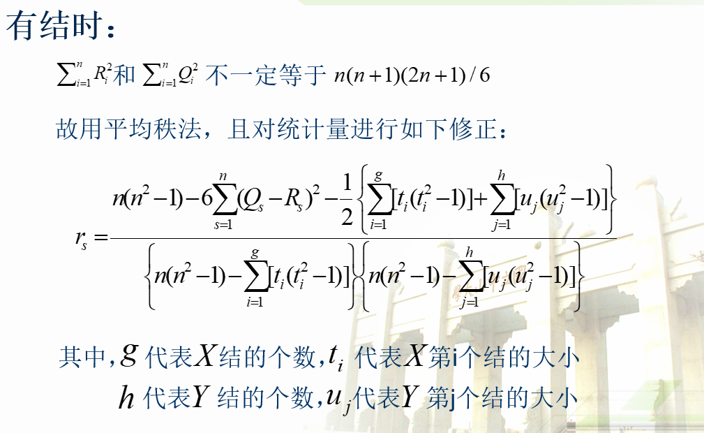
When there are no tie:
\[\sum_{i=1}^nR_i=\sum_{i=1}^nQ_i=\frac{n(n+1)}{2}, \sum_{i=1}^nR_i^2=\sum_{i=1}^nQ_i^2=\frac{n(n+1)(2n+1)}{6}\]
\[r_s=\frac{12\sum_{i=1}^nR_iQ_i}{n(n^2-1)}-3(\frac{n+1}{n-1})=1-\frac{6}{n(n^2-1)}\sum_{i=1}^n(R_i-Q_i)^2\]
In large sample case
\[E_0(r_s)=0, Var_0(r_s)=\frac{1}{n-1}\]
Note:
N1. Under null hypothesis, \(r_s\) is symmetric about 0
\[P_0(r_s\leq -x)=P_0(r_s\geq x)\]
N2. Under null hypothesis, \((R_1,...,R_n)\) and \((Q_1,...,Q_n)\) are independent and have uniform distribution on \(\mathscr{R}=\left\{(i_1,...,i_n)\right\}\)
\[\sum_{i=1}^nR_iQ_i=\sum_{j=1}^njQ_j\]
7.2 Kendall's tau test
\[\tau =2P\left\{(Y_2-Y_1)(X_2-X_1)>0\right\}-1\]
where \(P\left\{(Y_2-Y_1)(X_2-X_1)>0\right\}=P(X_2>X_1,Y_2>Y_1)+P(X_2<X_1,Y_2<Y_1)\)
hence, when \(X\) and \(Y\) are independent
\[P(X_2>X_1,Y_2>Y_1)=P(X_2>X_1)P(Y_2>Y_1)=\frac{1}{4}\]
\[P(X_2<X_1,Y_2<Y_1)=P(X_2<X_1)P(Y_2<Y_1)=\frac{1}{4}\]
Hypothesis: \(H_0: \tau=0\quad \Leftrightarrow \quad F_{XY}(x,y)=F_X(x)F_Y(y),\forall (x,y)\)
Test statistic:
\[\hat{\tau}=\frac{2}{n(n-1)}\sum_{1\leq i<j<n}sign((X_j-X_i)(Y_j-Y_i))\]
\[K=\frac{2}{n(n-1)}\sum_{1\leq i<j<n}sign((R_j-R_i)(Q_j-Q_i))\]
In large sample case
\[E_0(\hat{\tau})=0, Var_0(\hat{\tau})=\frac{2(2n+5)}{9n(n-1)}\]
Note:
N1. Another form of \(K\) can described with the number of concordant pairs and discordant paris.
\[K=\#\left\{\text{Concordant pairs}\right\}-\#\left\{\text{Discordant pairs}\right\}=K_1-K_2\]
N2. When there are no tie, \(K_1+K_2=\frac{n(n-1)}{2}\)
N3. Under null hypothesis, K has symmetric distribution about 0
\[P_0(K\leq -x)=P_0(K\geq x)\]
N4. According to empirical practice, \(\hat{\tau}\approx \frac{2}{3}r_s\)
7.3 Kolmogorov-Smirnov test
\[D=(\frac{mn}{gcd(m,n)})\sup_x|F_n(x)-G_m(x)|\]
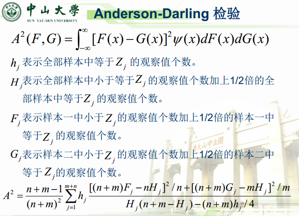
7.4 Anderson-Darling test
\[A^2(F,G)=\int_{-\infty}^{\infty}[F(x)-G(x)]^2\psi(x)dF(x)dG(x)\]
7.5 Cramer-von Mises test
When \(\psi(x)\equiv 1\) in AD test, it's a CVM test.
\[CVM=\frac{nm}{(n+m)^2}\sum_{i=1}^{m+n}[F_n(z_i)-G_m(z_i)]^2\]
7.6 Kruskal-Wallis test
Situation: There are k treatments with \(n_k\) observations respectively, whether the treatments are different?
Assumption:
A1. All observations are independent
A2. For fixed \(j\in \left\{1,...,k\right\}\), there are \(n_j\) observations \(\left\{X_{1j},...,X_{n_j,j}\right\}\sim F_j\)
A3. \(F_j(t)=F(t-\tau_j),-\infty<t<\infty\). F has an unknown median \(\theta\) and \(\tau_j\) is the unknown jth treatment effect
\[X_{ij}=\theta+\tau_j+e_{ij}\]
where \(\sum_{j=1}^k\tau_j=0\)
Hypothesis: \(H_0:\tau_1=\tau_2=...=\tau_k \Rightarrow F_1=...=F_k=F\)
Quick review on one-way ANOVA test:
Model:
\[y_{ij}=\mu+\alpha_i+e_{ij},e_{ij}\sim N(0,\sigma^2)\]
Breakdown the variance as
\[\sum_{i=1}^k\sum_{j=1}^{n_i}(y_{ij}-\bar{y})^2=\sum_{i=1}^k\sum_{j=1}^{n_i}(y_{ij}-\bar{y_i})^2+\sum_{i=1}^k\sum_{j=1}^{n_i}(\bar{y_i}-\bar{y})^2\]
or \(SST=SSW+SSB\). Then we can estimate the variance
\[\hat{\sigma_W}^2=MSW=\frac{SSW}{n-k}\]
\[\hat{\sigma_B}^2=MSB=\frac{SSB}{k-1}\]
The test statistic
\[F=\frac{MSB}{MSW}=\frac{\hat{\sigma_B}^2}{\hat{\sigma_W}^2}\sim F_{k-1,n-k}\]
Replace the sample value with its rank in its treatment group
\[(SSB)D=\sum_{j=1}^kn_j(\frac{R_j}{n_j}-R_{..})^2=\sum_{j=1}^kn_j(\frac{R_j}{n_j}-\frac{N+1}{2})^2\]
\[(SST)=\sum_{j=1}^k\sum_{i=1}^{n_j}(r_{ij}-R_{..})^2=\sum_{j=1}^k\sum_{i=1}^{n_j}r_{ij}^2-NR_{..}^2=\frac{N(N^2-1)}{12}\]
Test statistic:
\[H=\frac{12D}{N(N+1)}=(\frac{12}{N(N+1)}\sum_{j=1}^k\frac{R_j^2}{n_j})-3(N+1)\stackrel{D}{\sim}\chi^2(k-1)\]
Intuition: SSB has a asymptotic distribution of \(\chi^2(k-1)\)
Note: when \(k=2\), the test statistic is the same as Wilcoxon rank-sum test. Under null hypothesis
\[E_0(R_{.j})=\frac{N+1}{2},Var_0(R_{.j})=\frac{(N-n_j)(N+1)}{12n_j},Cov_0(R_{.i},R_{.j})=\frac{-(N+1)}{12}\]
7.7 Friedman test
Quick review on two-way ANOVA test:
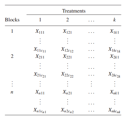
Situation: There are different n blocks and diifferent treatments, to see if the different block has additive effect and whether the treatment has effect on the result.
Assumptions:
A1. The \(N\) random variables are mutually independent
A2. For each fixed \((i,j)\), the \(c_{ij}\) random variables \((X_{ij1},...,X_{ijc_{ij}})\) are a random sample from a continuous distribution with distribution function \(F_{ij}\)
A3. \(F_{ij}(u)=F(u-\beta_i-\tau_j),-\infty<u<\infty\) F has an unknown median \(\theta\), \(\beta_i\) is the unknown additive effect contributed by block i, and \(\tau_j\) is the unknown jth treatment effect
#TODO: two-way ANOVA statistic
Denote \(r_{ij}\) the rank of \(X_{ij}\) in the \(i\)th block,\(i\in\left\{1,...,n\right\}, j\in\left\{1,...,k\right\}\), then
\[R_j=\sum_{i=1}^nr_{ij}\quad \text{and}\quad R_{.j}=\frac{R_j}{n}\]
Hypothesis: \(H_0:\tau_1=\tau_2=...=\tau_k \Rightarrow F_1=...=F_k=F\)
Test statistic:
\[ \begin{aligned} S=\frac{SSt}{SSe}&=\frac{12n}{k(k+1)}\sum_{j=1}^k(R_{.j}-\frac{k+1}{2})^2\\ &=[\frac{12}{nk(k+1)}\sum_{j=1}^kR_j^2]-3n(k+1)\sim\chi^2_{k-1} \end{aligned} \]
7.8 Page test
Situation: Assume that the additive effect of the blocks has a certain trend.
Hypothesis: \(H_0:\tau_1=\tau_2=...=\tau_k \quad v.s.\quad H_1:\tau_1\leq\tau_2\leq...\leq\tau_k\)
Test statistic:
\[L=\sum_{j=1}^kjR_j\]
under the null hypothesis:
\[E_0(L)=\frac{nk(k+1)^2}{4},Var_0(L)=\frac{nk^2(k+1)^2}{144}\]