生物统计

生物统计课程内容整理，参考教材：Fundamentals of Biostatistics(7th edition)

Lecture 1 Intro

1.1 Randomized Clinical Trial (RCT)

Definition: RCT is a type of research design used for comparing different treatments(especially to those samples with small size), in which patients are assigned to a particular treatment by some random mechanism to make sure that the characteristics of treatment groups are comparable.

1.1.1 Block Randomization

Defination: Block randomization is defined as follows in clinical trials comparing two treatments(A and B). A block size of \(2n\) is determined in advance according to the sample size, then assigned randomly \(n\) patients to treatment A, \(n\) patients to treatment B. (this can also be used in clinical trials with more than two treatment groups)

By doing so, we can obtain equal size treatment groups and this ensures comparability of treatment groups. One should be aware that the size of the block should be hidden, because one may know the treatment when the block size is fixed. (or use random-size blocks to avoid this)

1.1.2 Strafication

Defination: Strafication is the procedure that patients are subdivided into subgroups according to some important features, and separate randomization lists are maintained for each subgroup to ensure patient populations within each stratum.

1.1.3 Blinding

Deal with Placebo effect.

1.2 Descriptive Statistics

1.2.1 Measures of Location

Mean: \(\bar{x}=\frac{1}{n}\sum_{l=1}^nx_l\)

Median = $ \begin{cases} X_{((n+1)/2)}&\ (X_{(n/2)}+X_{(n/2+1)})& \end{cases} $

Mode: the most frequently occurring value

Geometric Mean: \(\overline{\log x}=\frac{1}{n}\sum_{l=1}^n\log x_l\)

1.2.2 Measures of Spread

Range: \(x_{\max}-x_{\min}\)

\[ \text{Quantiles = }\begin{cases} X_{(\lceil np\rceil)}&\text{if np is not an integer,}\\ (X_{(np)}+X_{(np+1)})/2 & \text{if np is an integer.} \end{cases} \]

Variance: \(s^2=\frac{\sum_{i=1}^n(x_i-\bar{x})^2}{n-1}\)

Standard Deviation: \(s=\sqrt{\frac{\sum_{i=1}^n(x_i-\bar{x})^2}{n-1}}\)

The Coefficient of Variation: \(CV=\dfrac{s}{\bar{x}}\times 100\%\)

1.2.3 Graphic Methods

• Bar Graphs
• Box Plots
• Scatter Plots

1.3 ROC curve

1.3.1 Hypothesis Testing

Hypothesis testing is concerned with making decisions using data. The null hypothesis is assumed true and statistical evidence is required to reject it in favor of a research of alternative hypothesis.

There are four possible outcomes:

1.3.1

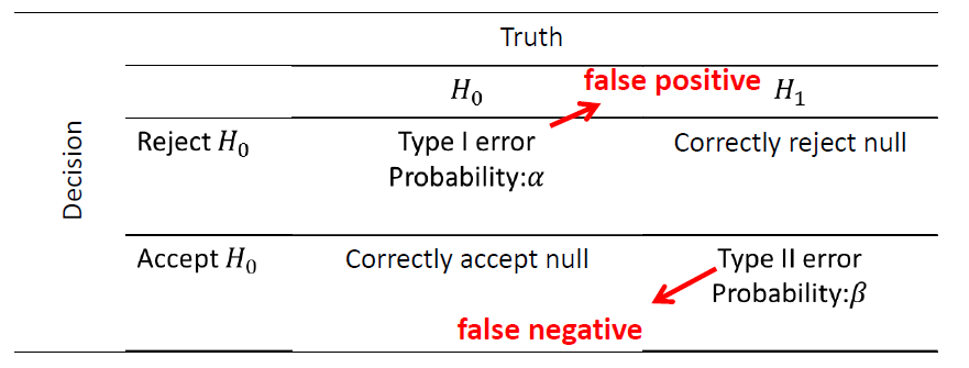
The general aim in hypothesis testing is to use statistical tests that make \(\alpha\) and \(\beta\) as small as possible.(genral strategy is to fix \(\alpha\) at some specific level and use the test that minimizes \(\beta\))

• making \(\alpha\) small involves rejecting \(H_0\) less often
• making \(\beta\) small involves accepting \(H_0\) less often

1.3.2 Sensitivity and Specificity

When assessing the diagnostic performance, "accuracy" number can be very misleading due to the low probability of occurance for some rare diseases. The probability of symptom is present that the person has a disease should be taken into account.

1.3.2

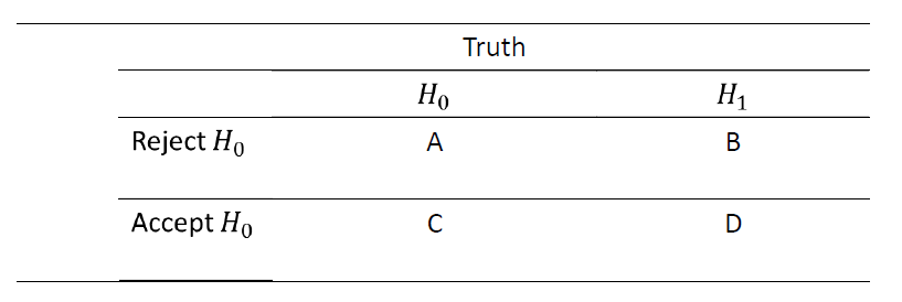
Sensitivity: the probability that the symptom is present given that the person has a disease. i.e.sensitivity = \(P(rejected|H_1)=\dfrac{B}{B+D}\), proportion of correctly rejected case to all H1 cases

Specificity: the probability that the symptom is not present given that the person does not have a disease. i.e. specificity = \(P(not\ rejected|H_0)=\dfrac{C}{A+C}\), proportion of correctly accepted case to all H0 cases

e.g. Disease: lung canser, Symptom: cigarette smoking.

If we assume that 90% of people with lung cancer and 30% of people without lung cancer are smokers, then sensitivity=.9, specificity=.7

False negative: a negative test result when the disease or condition being tested for is actually present.(\(\beta\), i.e. the test failed to identify the negative outcome, accept H0 when the truth is H1)

False positive: a positive test result when the disease or condition being tested for is not actually present.(\(\alpha\), i.e. the test failed to identify the positive outcome, reject H0 when the the truth is H0)

Positive Predictive Value(PPV): \(PPV=P(H_1|rejected)=\dfrac{B}{A+B}\)

Negative Predictive Value(NPV): \(NPV=P(H_0|not\ rejected)=\dfrac{C}{C+D}\)

Prevalence: probability of currently having the disease.(#people have the disease/#number of people in the study)

As prevalence increases, PPV increases and NPV decreases.

Note: Positive test = reject H0, Negative test = accept H0

1.3.2

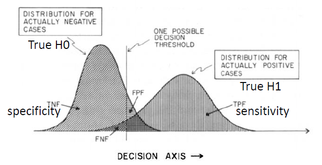
The measure with "true positive fraction" and "false positive fraction" are more meaningful than "accuracy" because they depend on the arbitrary selection of a decision threshold.

1.3.3 ROC Curve

Receiver Operating Characteristic(ROC) curve: indicating all possible combinations of the relative frequencies of the various kinds of correct and incorrect decisions. ROC Curve is a plot of the sensitivity versus (1-specificity), where the different points on the cureve correspond to different cutoff points used to designate test-positive.

Area Under Curve(AUC): Describe the "degree of separation", a summary of the overall diagnostic accuracy of the test.

AUC = 0.5 \(\Leftrightarrow\) random chance

AUC = 1.0 \(\Leftrightarrow\) all true-positives have higher values than any true-negatives

Lecture 2 Hypothesis Testing

Outline:

• Recap
• Hypothesis test under normal distribution
• Hypothesis test for binomial proportions
• Hypothesis test for the Poisson Distribution

2.1 Recap

P-value: the probability under the null hypothesis of obtaining evidence as extreme or more extreme thant would be observed by chance alone. If the P-value is small, then either \(H_0\) is true and we have observed a rare event or \(H_0\) is false.(set a level of \(\alpha\) to judge the significance)

Power: \(1-\beta = P(\text{reject}\ H_0|H_1)\)

2.2 Hypothesis test under normal distribution

2.2.1 One-sample test for the mean

Hypothesis: \(H_0:\mu=\mu_0\quad v.s.\quad H_1:\mu\not ={\mu_0}\)

Test statistic:

• t test: \(t=\frac{\bar{X}-\mu_0}{S/\sqrt{n}}\) (with \(\sigma\) unknown)
• z test: \(t=\frac{\bar{X}-\mu_0}{\sigma/\sqrt{n}}\) (with \(\sigma\) known)

Power for z-test (with \(\sigma\) known)

\[ \begin{aligned} 1-\beta &= P(\frac{|\bar{X}-\mu_0|}{\sigma/\sqrt{n}}>z_{1-\alpha/2}|\mu=\mu_1)\\ &= P(\frac{\bar{X}-\mu_1}{\sigma/\sqrt{n}}>z_{1-\alpha/2}+\frac{\mu_0-\mu_1}{\sigma/\sqrt{n}})+P(\frac{\bar{X}-\mu_1}{\sigma/\sqrt{n}}<z_{\alpha/2}+\frac{\mu_0-\mu_1}{\sigma/\sqrt{n}})\\ &=1-\Phi(z_{1-\alpha/2}+\frac{\mu_0-\mu_1}{\sigma/\sqrt{n}})+\Phi(z_{\alpha/2}+\frac{\mu_0-\mu_1}{\sigma/\sqrt{n}})\\ &=\Phi(-z_{1-\alpha/2}+\frac{\mu_1-\mu_0}{\sigma/\sqrt{n}})+\Phi(-z_{1-\alpha/2}+\frac{\mu_0-\mu_1}{\sigma/\sqrt{n}})\\ &\approx\Phi(-z_{1-\alpha/2}+\frac{|\mu_0-\mu_1|}{\sigma/\sqrt{n}}) \end{aligned} \]

Sample-size for z-test (with \(\sigma\) known)

\[z_{1-\beta}=-z_{1-\alpha/2}+\frac{|\mu_0-\mu_1|}{\sigma/\sqrt{n}}\]

\[n=\frac{\sigma^2(z_{1-\beta}+z_{1-\alpha/2})^2}{(\mu_0-\mu_1)^2}\]

Power for t-test (with \(\sigma\) unknown)

Since we have \(\frac{S}{\sigma}=\sqrt{\frac{(n-1)S^2}{\sigma^2}/(n-1)}=\sqrt{V/r},V\sim\chi^2(n-1)\) and \(\frac{\bar{X}-\mu_1}{\sigma/\sqrt{n}}\sim N(0,1)\)

\[ \frac{\bar{X}-\mu_0}{S/\sqrt{n}}=\frac{\frac{\bar{X}-\mu_1}{\sigma/\sqrt{n}}+\frac{\mu_1-\mu_0}{\sigma/\sqrt{n}}}{S/\sigma}\stackrel{H_1}{\sim}t_{n-1,ncp}\]

where \(ncp=\frac{\mu_1-\mu_0}{\sigma/\sqrt{n}}\).

\[ \begin{aligned} 1-\beta&=P(\frac{|\bar{X}-\mu_0|}{\sigma/\sqrt{n}}>t_{1-\alpha/2}(n-1)|\mu=\mu_1)\\ &=P(\frac{\bar{X}-\mu_0}{\sigma/\sqrt{n}}>t_{1-\alpha/2}(n-1)|\mu=\mu_1)+P(\frac{\bar{X}-\mu_0}{\sigma/\sqrt{n}}<t_{\alpha/2}(n-1)|\mu=\mu_1)\\ &=1-t_{n-1,ncp}(t_{1-\alpha/2}(n-1))+t_{n-1,ncp}(t_{\alpha/2}(n-1)) \end{aligned} \]

Usually, we take only one tail to calculate the power. We have

\[1-\beta \approx 1-t_{n-1,ncp}(t_{1-\alpha}(n-1))\]

Sample-size for t-test (with \(\sigma\) unknown)

With the required \(\beta\), solve \(t_{\beta,ncp}(n-1)=t_{1-\alpha}(n-1)\) to obtain the sample size.

CI width: Calculated based on \(CI=\bar{x}\pm \frac{s}{\sqrt{n}}t_{1-\alpha/2}(n-1),\ L=\frac{2s}{\sqrt{n}}t_{1-\alpha/2}(n-1)\) (similarly to z-test)

2.2.2 One-sample test for the Variance

Hypothesis: \(H_0:\sigma^2=\sigma^2_0\quad v.s.\quad H_1:\sigma^2\not ={\sigma^2_0}\)

Test statistic:

\[X^2=\frac{(n-1)s^2}{\sigma^2}\sim\chi^2(n-1)\]

2.3 Hypothesis test for binomial proportions

Assume that \(X_i\sim B(n,p)\)

Hypothesis: \(H_0:p=p_0\quad v.s.\quad H_1:p\not ={p_0}\)

The Score test statistic:

\[t = \frac{\hat{p}-p_0}{\sqrt{p_0(1-p_0)/n}}\sim N(0,1)\]

The Wald test statistic:

\[t = \frac{\hat{p}-p_0}{\sqrt{\hat{p}(1-\hat{p})/n}},\quad t^2\sim \chi^2(1)\]

Exact binomial tests: Consider calculating an exact P-value.

Remark: The difference of the Score test and the Wald test:

• the Score test: \(t=\frac{\hat{\theta_0}-\mu_{\theta_0}}{\sqrt{Var(\theta_0)}}\)
• the Wald test: \(t=\frac{\hat{\theta_0}-\mu_{\theta_0}}{\sqrt{Var\hat{\theta}}}\)

2.4 Hypothesis test for the Poisson Distribution

Assume that \(X_i\sim Poi(\mu)\)

Hypothesis: \(H_0:\mu=\mu_0\quad v.s.\quad H_1:\mu\not ={\mu_0}\)

Test statistic:

\[X^2=\frac{(x-\mu_0)^2}{\mu_0}\stackrel{H_0}{\sim}\chi^2(1)\]

Lecture 3 Hypothesis Testing: Two-sample Inference

Outline:

• Introduction
• Paired sample
• Two independent groups
  • Two sample t-test with equal variances
  • Testing for the equality of two variances
  • Two sample t-test with unequal variances
• Power analysis and Sample-size determination

3.1 Introduction

In a two-sample hypothesis testing problem, the underlying parameters of two different populations, neither of whose values is assumed known, are compared.

Longitudinal Study: (follow-up study)same group of people is followed overtime. i.e.paired sample

Cross-Sectional Study: the participants are seen only one point in time. i.e.independent sample

3.2 Paired sample(The paired t-test)

Denote \(d=X_1-X_2\) and do a one-sample t-test.

Hypothesis: \(H_0:\Delta=0\quad v.s.\quad H_1:\Delta\not ={0}\)

Test statistic:

\[t=\frac{\bar{d}}{s_d/\sqrt{n}}\stackrel{H_0}{\sim}t(n-1)\]

where \(s_d\) is the sample standard deviation of the observed differences. \[s_d=\sqrt{\dfrac{\sum_{i=1}^nd_i^2-\frac{(\sum_{i=1}^nd_i)^2}{n}}{n-1}}\]

3.3 Two independent groups

3.3.1 Two-sample t-test with equal variances

Assume that the underlying variances in the two groups are the same. \[\sigma_1^2=\sigma_2^2=\sigma^2\]

Then we have \(\bar{X_1}-\bar{X_2}\sim N[\mu_1-\mu_2,\sigma^2(\frac{1}{n_1}+\frac{1}{n_2})]\). We use the pooled estimate of the variance \(s^2\) instead of the unknown \(\sigma^2\)

Hypothesis: \(H_0:\mu_1=\mu_2\quad v.s.\quad H_1:\mu_1\not ={\mu_2}\)

Test statistic:

\[t=\frac{\bar{X_1}-\bar{X_2}}{S\sqrt{\frac{1}{n_1}+\frac{1}{n_2}}}\stackrel{H_0}{\sim}t(n_1+n_2-2)\]

where \(S^2\) is the pooled estimate of variance,

\[S^2=\frac{(n_1-1)s_1^2+(n_2-1)s_2^2}{n_1+n_2-2}\]

3.3.2 Testing for the equility of two variances

Hypothesis: \(\sigma_1^2=\sigma_2^2\quad v.s.\quad H_1:\sigma_1^2\not ={\sigma_2^2}\)

Test statistic:

\[F = \frac{s_1^2}{s_2^2}\stackrel{H_0}{\sim}F_{n_1-1,n_2-1}\]

It can be shown that

\[F_{d_1,d_2,p}=\frac{1}{F_{d_2,d_1,1-p}}\]

3.3.3 Two sample t-test with unequal variances

Assume that the two variances are significantly different.

Then we have \(\bar{X_1}-\bar{X_2}\sim N(\mu_1-\mu_2,\frac{\sigma_1^2}{n_1}+\frac{\sigma_2^2}{n_2})\)

Hypothesis: \(H_0:\mu_1=\mu_2\quad v.s.\quad H_1:\mu_1\not ={\mu_2}\)

Test statistic:

\[t=\frac{\bar{X_1}-\bar{X_2}}{\sqrt{\frac{S_1^2}{n_1}+\frac{S_2^2}{n_2}}}\stackrel{H_0}{\sim}t(d')\]

the approximate degrees of freedom \(d'\) is

\[d'=\dfrac{(\frac{s_1^2}{n_1}+\frac{s_2^2}{n_2})^2}{\frac{(s_1^2/n_1)^2}{n_1-1}+\frac{(s_2^2/n_2)^2}{n_2-1}}\]

3.4 Power analysis and Sample-size determination

Denote \(|\mu_1-\mu_2|=\Delta\), with significance level \(\alpha\),

\[ \begin{aligned} 1-\beta&=P(\frac{|\bar{X_1}-\bar{X_2}|}{\sqrt{\frac{\sigma_1^2}{n_1}+\frac{\sigma_2^2}{n_2}}}>z_{1-\alpha/2}|H_1)\\ &=P(\frac{\bar{X_1}-\bar{X_2}-(\mu_1-\mu_2)}{\sqrt{\frac{\sigma_1^2}{n_1}+\frac{\sigma_2^2}{n_2}}}>z_{1-\alpha/2}-\frac{\mu_1-\mu_2}{\sqrt{\frac{\sigma_1^2}{n_1}+\frac{\sigma_2^2}{n_2}}})+P(\frac{\bar{X_1}-\bar{X_2}-(\mu_1-\mu_2)}{\sqrt{\frac{\sigma_1^2}{n_1}+\frac{\sigma_2^2}{n_2}}}<z_{\alpha/2}-\frac{\mu_1-\mu_2}{\sqrt{\frac{\sigma_1^2}{n_1}+\frac{\sigma_2^2}{n_2}}})\\ &=\Phi(-z_{1-\alpha/2}+\frac{\mu_1-\mu_2}{\sqrt{\frac{\sigma_1^2}{n_1}+\frac{\sigma_2^2}{n_2}}})+\Phi(z_{\alpha/2}-\frac{\mu_1-\mu_2}{\sqrt{\frac{\sigma_1^2}{n_1}+\frac{\sigma_2^2}{n_2}}})\\ &\approx\Phi(-z_{1-\alpha/2}+\dfrac{\Delta}{\sqrt{\frac{\sigma_1^2}{n_1}+\frac{\sigma_2^2}{n_2}}}) \end{aligned} \]

then we have \(z_{1-\beta}=-z_{1-\alpha/2}+\dfrac{\Delta}{\sqrt{\frac{\sigma_1^2}{n_1}+\frac{\sigma_2^2}{n_2}}}\), suppose that \(n_2=kn_1\), it can be shown that

\[n_1=\frac{(\sigma_1^2+\frac{1}{k}\sigma_2^2))(z_{1-\alpha/2}+z_{1-\beta})^2}{\Delta^2}\]

Lecture 4 Nonparametric Methods

Outline:

• Types of data
• Nonparametric tests
• Sign test
• Wilcoxon Signed-rank test
• Sign sum test
• Sample size calculation

4.1 Types of Data

Cardinal data: on a scale where it is meaningful to measure the distance between possible data values. Interval scale data have the arbitrary zero point. (e.g.temperature) Ratio scale data have a fixed zero point. (e.g.weight)

Ordinal data: can be ordered but not have specific numeric values.

Categorical data: (Nominal data) data values can be classified into categories but the categories have no specific ordering.

4.2 The Sign Test

Situation: Exact value is not available (but which is better is known)

Target: Compare the performance of two groups

Intuition: Let \(d_i=a_i-b_i\), denote \(C=\sum_iI(d_i>0)\) the number of whom \(d_i>0\) out of the total of \(n\) people with nonzero \(d_i\), then C is binomial(n,p). If the two groups have similar performance, then the distribution of \(d_i\) should be symmetry.

Let \(\Delta\) be the population median of the \(d_i\).

Hypothesis: \(H_0:\Delta=0 \quad v.s.\quad H_1:\Delta\not ={0}\)

4.2.1 Normal-Theory Method

\[E(C)=\frac{n}{2}, \quad Var(C)=\frac{n}{4}\]

Test statistic:

\[Z=\frac{C-\frac{n}{2}}{\sqrt{\frac{n}{4}}}\stackrel{D}{\rightarrow}N(0,1)\]

Test statistic with continuity correction:

\[Z=\frac{C-\frac{n}{2}-0.5}{\sqrt{\frac{n}{4}}}\stackrel{D}{\rightarrow}N(0,1)\]

Note: Use this test only when \(n\geq 20\).

4.2.2 Exact Method

If \(C>\frac{n}{2},\quad p=2\times\sum_{k=C}^n\binom{n}{k}(\frac{1}{2})^n\).

If \(C<\frac{n}{2},\quad p=2\times\sum_{k=0}^C\binom{n}{k}(\frac{1}{2})^n\).

If \(C=\frac{n}{2},\quad p=1.0\).

4.3 Wilcoxon Signed-rank test

Situation: Exact value is available. Two groups of samples(paired)

Target: Compare the performance of two groups. Take "distance" into account.

Intuition: Let \(R_i=|d_i|=|a_i-b_i|\) and rank these values. Consider the rank sum of which \(d_i>0\). Since the rank sum outcome has equal probability, if the two groups have similar performance, the positive rank sum should be half of the total rank sum.

Denote \(W_+=\sum_{i=1}^nR_i\phi_i\), where \(R_i=|d_i|, \phi_i=I(d_i>0)\).

Since \(W=W_++W_-=\dfrac{n(n+1)}{2}\), under \(H_0\) with no ties :

\[E(W_+)=\frac{n(n+1)}{4},\quad Var(W_+)=\frac{n(n+1)(2n+1)}{24}\]

If there are ties :

\[Var(W_+)=\frac{n(n+1)(2n+1)}{24}-\sum_{g=1}^g\frac{t_i^3-t_i}{48}\]

4.4 Wilcoxon Rank-Sum Test (Mann-Whitney Test)

Situation: Two groups of samples(not paired). Treatment effect.

Target: Compare if a certain feature of the sample is significantly different.(if treatment effect exists)

Intuition: Discard the labels and rank all the observations. If treatment effect doesn't exist, the sum of the ranks in the first and the second treatment would be proportioned by the sample size.

Let \(X_1,X_2,...,X_{n_1}\sim F,Y_1,Y_2,...,Y_{n_2}\sim G\), denote the statistic

\[ \begin{aligned} W_X&=\sum_{i=1}^{n_1}rank(X_i)\\ &=\sum_{i=1}^{n_1}(\sum_{j=1}^{n_1}I(X_j\leq X_i)+\sum_{j=1}^{n_2}I(Y_j\leq X_i))\\ &=\frac{n_1(n_1+1)}{2}+\sum_{i=1}^{n_1}\sum_{j=1}^{n_2}I(Y_j\leq X_i) \end{aligned} \]

Here we have Mann-Whitney Statistic:

\[W_{YX}=\sum_{i=1}^{n_1}\sum_{j=1}^{n_2}I(Y_j\leq X_i)\]

Hypothesis: \(H_0:F(x)=G(x),\forall x \quad v.s.\quad H_1:F(x)\not =G(x), \exists x\)

Under \(H_0\), if there are no ties:

\[E(W_X)=\frac{n_1(n_1+n_2+1)}{2}, Var(W_X)=\frac{n_1n_2(n_1+n_2+1)}{12}\]

If there are ties:

\[Var(W_X)=\frac{n_1n_2(n_1+n_2+1)}{12}-\sum_{i=1}^g\frac{n_1n_2(t_i^3-t_i)}{12(n_1+n_2)(n_1+n_2+1)}\]

Note: Normal approximate should be used only if both \(n_1\) and \(n_2\) are at least 10.

Remark: Comparision of the Wilcoxon Signed rank test and Wilcoxon Rank sum test

• Singed rank: \(f(·)\) is symmetric around \(\Delta\)
• Rank sum: \(G(x)=F(x-\Delta)\) or \(Y=X+\Delta\)
• Hypothesis: \(H_0:\Delta=0\quad vs.\quad H_1:\Delta\not ={0}\)

4.5 Sample-size Calculation

4.5.1 Sign test

One-sample case: \(Z_1,Z_2,...,Z_n\sim f\), let \(\theta\) be the population median of the \(f(x)\).

\[H_0:\theta=0 \quad v.s. \quad H_1:\theta\not ={0}\]

\[\Leftrightarrow H_0:p=P(Z>0|Z\not ={0})=0.5 \quad v.s. \quad H_1:p\not ={0.5}\]

\[C=\sum_{i=1}^nI(Z_i>0)\] \[T=\frac{C-\frac{n}{2}}{\sqrt{\frac{n}{4}}}\stackrel{H_0}{\sim}N(0,1)\]

Under \(H_1\), \(C\sim B(n,p_1)\)

\[ \begin{aligned} 1-\beta&=P(T>z_{1-\frac{\alpha}{2}}|p=p_1)\\ &=P(\frac{C-np_1}{\sqrt{np_1(1-p_1)}}>\frac{\sqrt{n/4}}{\sqrt{np_1(1-p_1)}}z_{1-\alpha/2}+\frac{n/2-np_1}{\sqrt{np_1(1-p_1)}})\\ &\quad +P(\frac{C-np_1}{\sqrt{np_1(1-p_1)}}<\frac{\sqrt{n/4}}{\sqrt{np_1(1-p_1)}}z_{\alpha/2}+\frac{n/2-np_1}{\sqrt{np_1(1-p_1)}})\\ &=\Phi(\frac{-z_{1-\alpha/2}}{\sqrt{4p_1(1-p_1)}}-\frac{n/2-np_1}{\sqrt{np_1(1-p_1)}})+\Phi(\frac{z_{1-\alpha/2}}{\sqrt{4p_1(1-p_1)}}+\frac{n/2-np_1}{\sqrt{np_1(1-p_1)}})\\ &\approx\Phi(\frac{-z_{1-\alpha/2}}{\sqrt{4p_1(1-p_1)}}+\frac{n|0.5-p_1|}{\sqrt{np_1(1-p_1)}}) \end{aligned} \]

4.5.2 Wilcoxon Signed Rank test

One-sample case: \(Z_1,Z_2,...,Z_n\sim f\),\(f(·)\) is symmetric around \(\theta\)

\[H_0:\theta=0 \quad v.s. \quad H_1:\theta\not ={0}\]

Under \(H_1\),

\[ \begin{aligned} 1-\beta &= P(|W^*|>z_{1-\frac{\alpha}{2}}|\theta\not ={0})\\ &=P(\frac{W-(\frac{n_2(n_2+1)}{2}+n_1n_2p_1)}{\sigma_W}>\frac{z_{1-\frac{\alpha}{2}}\sqrt{\frac{n_1n_2(n_1+n_2+1)}{12}}+n_1n_2(0.5-p_1)}{\sigma_W})\\ &\qquad +P(\frac{W-(\frac{n_2(n_2+1)}{2}+n_1n_2p_1)}{\sigma_W}<\frac{z_{\frac{\alpha}{2}}\sqrt{\frac{n_1n_2(n_1+n_2+1)}{12}}+n_1n_2(0.5-p_1)}{\sigma_W})\\ &=\Phi(\frac{-z_{1-\frac{\alpha}{2}}\sqrt{\frac{n_1n_2(n_1+n_2+1)}{12}}-n_1n_2(0.5-p_1)}{\sigma_W})+\Phi(\frac{z_{\frac{\alpha}{2}}\sqrt{\frac{n_1n_2(n_1+n_2+1)}{12}}+n_1n_2(0.5-p_1)}{\sigma_W})\\ &\approx\Phi(\frac{-z_{1-\frac{\alpha}{2}}\sqrt{\frac{n_1n_2(n_1+n_2+1)}{12}}+n_1n_2|0.5-p_1|}{\sigma_W}) \end{aligned} \]

4.6 Some other topics

\[AUC = \frac{U}{n_1n_2}\]

Where U is the Mann-Whitney Statistic.

For random variables \(\xi=(X_1,...,X_{n_1},Y_1,...,Y_{n_2})\) and Z,

\(c-index = P(\xi_1<\xi_2|Z_1<Z_2)\Leftrightarrow P(\xi_1<\xi_2|Z_1=0,Z_2=1)\Leftrightarrow P(X_1<Y_1)\)

Lecture 5 Categorical Data

Outline:

• Two sample test for Binominal propotions
  • Normal theory approach
  • Contingency table approach
• Fisher's exact test
• McNemar's test
• Sample size and power estimation
• \(R\times C\) contingency tables
• Goodness of Fit
• The Kappa Statistic

5.1 Two-Sample Test for Binomial Proportions

Situation: Categorical data

Target: Figure out whether the difference is significant between two categories.

Hypothesis: \(H_0:p_1=p_2=p\quad v.s. \quad H_1:p_1\not ={p_2}\)

5.1.1 Normal-Theory Method

Intuition: Compare the difference between the sample proportions \((\hat{p_1}-\hat{p_2})\). If \(H_0\) is true, the difference should be small. The samples will be assumed large enough so that normal approximation is valid.

Under \(H_0\) : \[E(\hat{p_1}-\hat{p_2})=0 \quad std(\hat{p_1}-\hat{p_2})=\sqrt{pq(\frac{1}{n_1}+\frac{1}{n_2})}\]

Test statistic: \[z=\frac{\hat{p_1}-\hat{p_2}}{\sqrt{\hat{p}\hat{q}(\frac{1}{n_1}+\frac{1}{n_2})}}\sim N(0,1)\]

where \(\hat{p}=\dfrac{n_1\hat{p_1}+n_2\hat{p_2}}{n_1+n_2}=\dfrac{x_1+x_2}{n_1+n_2}, \hat{q}=1-\hat{p}.\)

Test statistic with continutiy correction :

\[z=\frac{|\hat{p_1}-\hat{p_2}|-(\frac{1}{2n_1}+\frac{1}{2n_2})}{\sqrt{\hat{p}\hat{q}(\frac{1}{n_1}+\frac{1}{n_2})}}\sim N(0,1)\]

Note: Use this test only when \(n_1\hat{p}\hat{q}\geq5\) and \(n_2\hat{p}\hat{q}\geq5\).

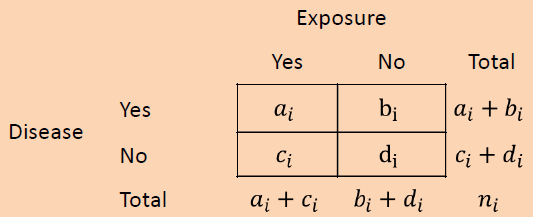
5.1.2 Contingency table approach

Intuition: Set up contingency table, apply chi-squared test.

• This test is called a test for homogeneity of binomial proportions. In this situation, one set of margins is fixed and the number of successes in each row is a random variable.

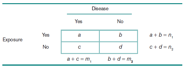
	Exposed	Unexposed	Total
Case	\(O_{11}\)	\(O_{12}\)	\(n_{1.}\)
Control	\(O_{21}\)	\(O_{22}\)	\(n_{2.}\)
Total	\(n_{.1}\)	\(n_{.2}\)	\(n_{..}\)

The expected number of units in the \((i,j)\) cell :

\[E_{ij}=\frac{n_{i.}n_{.j}}{n_{..}}\]

Test statistics:

\[\chi^2=\sum_{i,j}\frac{(O_{ij}-E_{ij})^2}{E_{ij}}\stackrel{H_0}\sim \chi^2_1\]

Test statistics with Yates' continuity correction :

\[\chi^2=\sum_{i,j}\frac{(|O_{ij}-E_{ij}|-0.5)^2}{E_{ij}}\stackrel{H_0}\sim \chi^2_1\]

Alternative form:

\[\chi^2=\frac{n_{..}(n_{11}n_{22}-n_{12}n_{21})^2}{n_{.1}n_{.2}n_{1.}n_{2.}}\]

Note: The test is used only when \(E_{ij}>5,\forall i,j.\)

5.1.3 More details about chi-squared

• The \(\chi^2\) statistic can be used
  • the rows are fixed (binomial)
  • the colomns are fixed (binomial)
  • the total sample size is fixed (multinomial)
  • none are fixed (Poisson)
• For a given set of data, any of these assumptions results in the same value for the statistic.
• \(df=n_{..}-1\)

5.2 Fisher's Exact Test

Situation: Categorical data, small samples

Target: Figure out whether the difference is significant between two categories.

Hypothesis: \(H_0:p_1=p_2=p\quad v.s. \quad H_1:p_1\not ={p_2}\)

Exact Probability of Obeserving a Table with a certain cell :

\[Pr(n_{11},n_{12},n_{21},n_{22})=\frac{n_{1.}!n_{2.}!n_{.1}!n_{.2}!}{n_{..}!n_{11}!n_{12}!n_{21}!n_{22}!}\]

Suppose we consider all possible tables with fixed row margins and fixed column margins. Then rearrange the rows and columns so that \(n_{1.}\leq n_{2.}, n_{.1}\leq n_{.2}\).

The random variable \(X\) denote the cell count in \((1,1)\) : \[Pr(X=a)=\frac{n_{1.}!n_{2.}!n_{.1}!n_{.2}!}{n_{..}!a!(n_{1.}-a)!(n_{.1}-a)!(n_{.2}-n_{1.}+a)!}\stackrel{H_0}{\sim}Hypergeometric(n_{1.},n_{2.},n_{..})\]

Also, under \(H_0\) :

\[E(X)=\frac{n_{1.}n_{.1}}{n_{..}},\quad Var(X)=\frac{n_{1.}n_{2.}n_{.1}n_{.2}}{n_{..}^2(n_{..}-1)}\]

Enumerate all possible tables and compute the exact probability of each table using the formula above. Calculate the p-value(two-tailed test) :

\[p-value = 2\times \min [Pr(0)+Pr(1)+...+Pr(a),Pr(a)+Pr(a+1)+...+Pr(k),0.5]\]

5.3 McNemar's test

Situation: Samples are paired and dependent.

Target: Figure out whether the difference is significant between two categories. Here, the two categories are dependent.

Type A/Type B	Case	Control	Total
Case	\(n_{11}\)	\(n_{12}\)	\(n_1\)
Control	\(n_{21}\)	\(n_{22}\)	\(n_2\)
Total	\(m_1\)	\(m_2\)	\(n\)

• Concordant pair : matched pair in which the outcome is the same for each member of the pair. i.e. \(n_{11}\) and \(n_{22}\).
• Discordant pair : matched pair in which the outcomes differ for the member of the pair, which shows the difference between the categories. i.e. \(n_{12}\) and \(n_{21}\).

Suppose that of \(n_D\) discordant pairs, \(n_A\) are type A.

Hypothesis: \(H_0 : p=\frac{1}{2} \quad v.s. \quad H_1:p\not ={\frac{1}{2}}\), where \(p=\dfrac{n_A}{n_D}\).

Under \(H_0\), \(n_A\sim Binomial(n_D,0.5)\) :

\[E(n_A)=\frac{n_D}{2},\quad Var(n_A)=\frac{n_D}{4}\]

Test statistic:

\[\chi^2=\frac{(n_A-\frac{n_D}{2})^2}{\frac{n_D}{4}}\stackrel{H_0}{\sim}\chi^2_1\]

Alternative form:

\[\chi^2=\frac{(n_A-n_B)^2}{n_D}\]

Test statistic with continutiy correction :

\[\chi^2=\frac{(|n_A-\frac{n_D}{2}|-0.5)^2}{\frac{n_D}{4}}\stackrel{H_0}{\sim}\chi^2_1\]

Note: Use this test only if \(n_D\geq20\).

5.4 Sample size and power estimation

5.4.1 Two proportions comparision

Denote \(\Delta=|p_2-p_1|\), \(p_1,p_2\) = projected true probabilities of success in the two groups, suppose that \(n_2=kn_1\), then \(\bar{p}=\frac{p_1+kp_2}{1+k}\), with significance level \(\alpha\), the power is

\[ \begin{aligned} 1-\beta&=P(\frac{|\hat{p_1}-\hat{p_2}|}{\sqrt{\hat{p}(1-\hat{p})(\frac{1}{n_1}+\frac{1}{n_2})}}>z_{1-\alpha/2}|H_1)\\ &=P(\frac{\hat{p_1}-\hat{p_2}-(p_1-p_2)}{\sqrt{\frac{p_1q_1}{n_1}+\frac{p_2q_2}{n_2}}}>z_{1-\alpha/2}\frac{\sqrt{\bar{p}\bar{q}(1/n_1+1/n_2)}}{\sqrt{\frac{p_1q_1}{n_1}+\frac{p_2q_2}{n_2}}}-\frac{p_1-p_2}{\sqrt{\frac{p_1q_1}{n_1}+\frac{p_2q_2}{n_2}}})\\ &\qquad +P(\frac{\hat{p_1}-\hat{p_2}-(p_1-p_2)}{\sqrt{\frac{p_1q_1}{n_1}+\frac{p_2q_2}{n_2}}}<z_{\alpha/2}\frac{\sqrt{\bar{p}\bar{q}(1/n_1+1/n_2)}}{\sqrt{\frac{p_1q_1}{n_1}+\frac{p_2q_2}{n_2}}}-\frac{p_1-p_2}{\sqrt{\frac{p_1q_1}{n_1}+\frac{p_2q_2}{n_2}}})\\ &=\Phi(-z_{1-\alpha/2}\frac{\sqrt{\bar{p}\bar{q}(1/n_1+1/n_2)}}{\sqrt{\frac{p_1q_1}{n_1}+\frac{p_2q_2}{n_2}}}+\frac{p_1-p_2}{\sqrt{\frac{p_1q_1}{n_1}+\frac{p_2q_2}{n_2}}})+\Phi(z_{\alpha/2}\frac{\sqrt{\bar{p}\bar{q}(1/n_1+1/n_2)}}{\sqrt{\frac{p_1q_1}{n_1}+\frac{p_2q_2}{n_2}}}-\frac{p_1-p_2}{\sqrt{\frac{p_1q_1}{n_1}+\frac{p_2q_2}{n_2}}})\\ &\approx\Phi(-z_{1-\alpha/2}\frac{\sqrt{\bar{p}\bar{q}(1/n_1+1/n_2)}}{\sqrt{\frac{p_1q_1}{n_1}+\frac{p_2q_2}{n_2}}}+\frac{\Delta}{\sqrt{\frac{p_1q_1}{n_1}+\frac{p_2q_2}{n_2}}}) \end{aligned} \]

We have \(z_{1-\beta}=\frac{\Delta}{\sqrt{\frac{p_1q_1}{n_1}+\frac{p_2q_2}{n_2}}}-z_{1-\alpha/2}\frac{\sqrt{\bar{p}\bar{q}(1/n_1+1/n_2)}}{\sqrt{\frac{p_1q_1}{n_1}+\frac{p_2q_2}{n_2}}}\), it can be shown that

\[n_1=\frac{[\sqrt{\bar{p}\bar{q}(1+\frac{1}{k})}z_{1-\alpha/2}+\sqrt{p_1q_2\dfrac{p_2q_2}{k}}z_{1-\beta}]^2}{\Delta^2}\]

5.4.2 Paired samples

Denote the specific alternative \(p=p_A\), with significance level \(\alpha\)

Since \(\hat{p_A}\sim N(p_A,\frac{p_Aq_A}{n_D})\)

\[ \begin{aligned} 1-\beta&=P(\frac{|n_A-\frac{n_D}{2}|}{\sqrt{\frac{n_D}{4}}}>z_{1-\alpha/2}|H_1)\\ &=P(\frac{\hat{p_A}-\frac{1}{2}}{\sqrt{\frac{1}{4n_D}}}>z_{1-\alpha/2}|H_1)+P(\frac{\hat{p_A}-\frac{1}{2}}{\sqrt{\frac{1}{4n_D}}}<z_{\alpha/2}|H_1)\\ &=P(\frac{\hat{p_A}-p_A}{\sqrt{\frac{p_Aq_A}{n_D}}}>\frac{z_{1-\alpha/2}}{\sqrt{4p_Aq_A}}+\frac{\frac{1}{2}-p_A}{\sqrt{\frac{p_Aq_A}{n_D}}})+P(\frac{\hat{p_A}-p_A}{\sqrt{\frac{p_Aq_A}{n_D}}}<\frac{z_{\alpha/2}}{\sqrt{4p_Aq_A}}+\frac{\frac{1}{2}-p_A}{\sqrt{\frac{p_Aq_A}{n_D}}})\\ &=\Phi(\frac{-z_{1-\alpha/2}}{\sqrt{4p_Aq_A}}-\frac{\frac{1}{2}-p_A}{\sqrt{\frac{p_Aq_A}{n_D}}})+\Phi(\frac{z_{\alpha/2}}{\sqrt{4p_Aq_A}}+\frac{\frac{1}{2}-p_A}{\sqrt{\frac{p_Aq_A}{n_D}}})\\ &\approx\Phi(\frac{-z_{1-\alpha/2}}{\sqrt{4p_Aq_A}}+\frac{|\frac{1}{2}-p_A|}{\sqrt{\frac{p_Aq_A}{n_D}}}) \end{aligned} \]

We have \(z_{1-\beta}=\frac{-z_{1-\alpha/2}}{\sqrt{4p_Aq_A}}+\frac{|\frac{1}{2}-p_A|}{\sqrt{\frac{p_Aq_A}{n_D}}}\), it can be shown that

\[n=\frac{(z_{1-\alpha/2}+2z_{1-\beta}\sqrt{p_Aq_A})^2}{4(p_A-0.5)^2p_D}\]

where \(p_D=\frac{n_D}{n}\) is projected proportion of discordant pairs among all pairs. \(n\) matched pairs are required.

5.4.3 Compliance

Definition: Compliance describes the degree to which a patient correctly follows medical advice.

Two types of noncompliance to consider:

• dropout rate \(\lambda_1\): the proportion of participants who fail to actually receive the active treatment
• drop-in rate \(\lambda_2\): the proportion of participants in the placebo group who actually receive the active treatment outside the study protocol

under the assumption of perfect compliance:

• \(p_1\)=incidence of disease among participants who actually receive treatment
• \(p_2\)=incidence of disease among participants who don't receive treatment

Assuming that compliance is not perfect:

• \(p_1^*\)=observed rate of disease in the treatment groups
• \(p_2^*\)=observed rate of disease in the placebo groups

then we have

\[p_1^*=p_1(1-\lambda_1)+p_2\lambda_1,\quad p_2^*=p_2(1-\lambda_2)+p_1\lambda_2\]

5.5 \(R\times C\) contingency tables

An \(R\times C\) contingency table is a table with \(R\) rows and \(C\) columns, which displays the relationship between two variables.

Test statistics:

\[\chi^2=\sum_{i,j}\frac{(O_{ij}-E_{ij})^2}{E_{ij}}\stackrel{H_0}\sim \chi^2_{(R-1)\times(C-1)}\]

Chi-square test for trend:

To test if there is a trend between two groups for all variables. Assign each group with a numeric attribute (mean or other particular numbers), which is called Score variable \(S_i\)

Hypothesis: \(H_0:\)There is no trend among the \(p_i's\quad v.s.\quad H_1:\)The trend exists,\(p_i=\alpha+\beta S_i\)

Test statistic:

\[\chi^2_\text{trend}=\frac{(\sum x_iS_i-x\bar{S})^2}{\bar{p}(1-\bar{p})(\sum n_iS_i^2-(\sum n_iS_i)^2)/n}\stackrel{H_0}{\sim}\chi^2_1\]

5.6 Goodness of Fit

Test statistics:

\[\chi^2=\sum_{i,j}\frac{(O_{ij}-E_{ij})^2}{E_{ij}}\stackrel{H_0}\sim \chi^2_{g-1-k}\]

where g=the number of groups, k=number of paramters to be estimated

5.7 The Kappa Statistic

The Cohen's Kappa Statistic measures the agreement/association between two variables

\[\kappa = \frac{p_o-p-e}{1-p_e}\]

where

• \(p_o=\) observed probability of concordance between the two surveys
• \(p_e=\) expected probability of concordance between the two surveys, \(p_e=\sum a_ib_i\), where \(a_i,b_i\) is the marginal probabilities of the two surveys.

Test statistic:

\[z=\frac{\kappa}{se(\kappa)}\]

where

\[se(\kappa)=\frac{1}{(1-p_e)\sqrt{n}}\sqrt{p_e+p_e^2-\sum a_ib_i(a_i+b_i)}\]

Lecture 6 Regression and Correlation Methods

Outline:

• Regression Topic
• Correlation coefficient
  • Pearson correlation coefficient
  • Spearman rank correlation coefficient
  • Kendall's Tau

6.1 Regression Topic

Refer to Applied Linear Regression course.

6.2 Correaltion coefficient

6.2.1 Pearson correlation coefficient

The sample Pearson correlation coefficient is defined by

\[r=\frac{L_{xy}}{\sqrt{L_{xx}L_{yy}}}\]

where \(L_{xy}=\sum(x_i-\bar{x})(y_i-\bar{y}), L_{xx}=\sum(x_i-\bar{x})^2, L_{yy}=\sum(y_i-\bar{y})^2\)

Also

\[r=\frac{s_{xy}}{\sqrt{s_{xx}s_{yy}}}\]

The regression model \(Y=\beta_0+\beta_1X\), then

\[\beta_1=\frac{L_{xy}}{L_{xx}}=\sqrt{\frac{L_{yy}}{L_{xx}}}\times r\]

Note:

1. The regression coefficient is based on the normal distribution assumption, which means that the \(Y_i\) should follow a normal distribution. Also, the relationship between correlation coefficient and regression coefficient depends on that.
2. r does not change if the units of measurement are changed, while \(\beta_1\) depends.

• Predict one variable from another \(\Rightarrow\) regressioon coefficient
• Describe the linear relationship between two variables \(\Rightarrow\) correlation coefficient

6.2.2 Spearman rank correlation coefficient

\[r_s=\frac{R_{xy}}{\sqrt{R_{xx}\times R_{yy}}}\]

where the R's are computed from the ranks rather than from the actual scores

Hypothesis: \(H_0:\rho=0\quad v.s. \quad H_1:\rho\not ={0}\)

Test statistic:

\[t_s=\frac{r_s\sqrt{n-2}}{\sqrt{1-r_s^2}}\stackrel{H_0}{\sim}t_{n-2}\]

6.2.3 Kendall's Tau

The Kendall's Tau is based on the number of concordant and discordant pairs.(describe the trend of the paired data)

\[\hat{\tau}=\frac{\sum_{1\leq i<j<n}sign((X_j-X_i)(Y_j-Y_i))}{\frac{n(n-1)}{2}}\]

another form:

\[\tau=\frac{K_1-K_2}{\frac{n(n-1)}{2}}\]

where \(K_1\) is the number of concordant pairs and \(K_2\) is the number of discordant paris

Lecture 7 Fixed Effects Models

Outline:

• One-Way ANOVA--Fixed Effects
  • One-way ANOVA
  • Post-hoc Test After One-way ANOVA
• Two-Way ANOVA
• The Kruskal-Wallis Test

7.1 One-Way ANOVA

\[ y_{ij}=\mu+\alpha_i+e_{ij},e_{ij}\sim N(0,\sigma^2) \]

Constraint: \(\sum_{i=1}^k \alpha_i=0\)

• \(\mu\) is the underlying mean of all groups taken together
• \(\alpha_i\) is the difference between the mean of the ith group and the overall mean
• \(e_{ij}\) is the random error about the mean \(\mu+\alpha_i\) for an individual observation from the ith group

Situation: whether there are differences between groups

7.1.1 F-test for ANOVA

Hypothesis: \(H_0:\alpha_1=...=\alpha_k=0\quad v.s.\quad H_1:\alpha_j\neq 0,\exists j\)

\(SSTO=\sum_{i=1}^k\sum_{j=1}^{n_i}(y_{ij}-\bar{y})^2\sim\sigma^2\chi^2(n-1)\)

\(SSW=\sum_{i=1}^k\sum_{j=1}^{n_i}(y_{ij}-\bar{y_i})^2\sim\sigma^2\chi^2(n-k)\)

\(SSB=\sum_{i=1}^k\sum_{j=1}^{n_i}(\bar{y_i}-\bar{y})^2=\sum_{i=1}^kn_i(\bar{y_i}-\bar{y})^2\sim\sigma^2\chi^2(k-1,\lambda)\)

Test statistic:

\[ F^*=\frac{MSB}{MSW}=\frac{SSB/(k-1)}{SSW/(n-k)}\stackrel{H_0}{\sim}F(k-1,n-k) \]

7.1.2 t-test for Comparison(LSD)

Hypothesis: \(H_0:\alpha_1=\alpha_2\quad v.s. \quad H_1:\alpha_1\neq\alpha_2\)

Test Statistic:

\[ t^*=\frac{\bar{y_1}-\bar{y_2}}{s\sqrt{\frac{1}{n_1}+\frac{1}{n_2}}}\stackrel{H_0}{\sim}t_{n-k} \]

where \(s=\hat{\sigma}_W^2=MSW\) is the "pooled" sample estimate of the common variance

7.1.3 Multiple Comparison

For more than one group, performing individual comparisons require multiple hypothesis tests (for \(n\) independent tests, TypeI error probability is \(1-(1-0.05)^n\))

Familty Wise typeI Error Rate(FWER):

\[ FWER=Pr(\cup_{i=1}^n A_i)=1-\prod_{i=1}^n(1-\alpha_i) \]

where \(A_i\) is typeI error occurs in the ith hypothesis testing

Bonferroni Adjustment: A possible correction for multiple comparisons

\[ \alpha^*=\frac{\alpha}{\binom{k}{2}} \]

where \(\alpha\) is FWER

Bonferroni Adjustment ensures overall typeI error rate does not exceed \(\alpha=0.05\), but it's too conservative

False-Discovery Rate(FDR): attempts to control the proportion of false positive results among reported statistically significant results

7.1.3

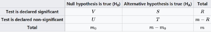
\[ Q=\begin{cases} V/R,&R>0\\ 0,&R=0 \end{cases} \]

\[ FDR=E(Q)=E(V/R|R>0)Pr(R>0) \]

since \(FWER=Pr(V\geq 1)\), it's found that \(FDR\leq FWER\) (when \(m=m_0\) the equality holds). Thus controlling FDR may gain power comparing to controlling FWER.

FDR Testing Procedure:

1. Renumber all \(p_i\) so that \(p_1\leq p_2\leq...\leq p_k\)
2. Define \(q_i=kp_i/i\), where \(i\) is the rank of p-values among the \(k\) tests
3. Let \(FDR_i=\min(q_i,...,q_k)\)
4. Find the largest \(i\) such that \(FDR_i<FDR_0\)
5. reject all \(1,...,i\) hypotheses

7.2 Two-Way ANOVA

• Main Effect: effect of one treatment variable considered in isolation
• Interaction Effect: the effect of one variable depends on the level of the other variable

\[ y_{ijk}=\mu+\alpha_i+\beta_j+\gamma_{ij}+e_{ijk},e_{ijk}\sim N(0,\sigma^2) \]

• \(\alpha_i\) the effect of row group
• \(\beta_j\) the effect of column group
• \(\gamma_{ij}\) the interaction effect between row group and column group

Constraint:

• \(\sum\alpha_i=\sum\beta_j=0\)
• \(\sum_i\gamma_{ij}=0,\sum_j\gamma_{ij}=0\)

(Refer to PPT Lecture7,page44)

7.3 Kruskal-Wallis Test

A nonparametric alternative to the one-way ANOVA

\[ H^*=\frac{12}{N(N+1)}\sum n_i(\bar{R_i}-\bar{R})^2\stackrel{H_0}{\sim}\chi_{k-1}^2 \]

Lecture 8 Random Effects Models

Outline:

• One-Way ANOVA--Random Effects
• Meta Analysis
• Mixed Model

8.1 Random-Effects One-way ANOVA

\[ y_{ij}=\mu+\alpha_i+\epsilon_{ij} \]

• \(\alpha_i\) is the between-subject variability, \(\alpha_i\sim N(0,\sigma_A^2)\)
• \(e_{ij}\) is the within-subject variability, \(e_{ij}\sim N(0,\sigma^2)\) and independent of \(\alpha_i,e_{ij}\)

Hypothesis: \(H_0:\sigma_A^2=0\quad v.s.\quad H_1:\sigma_A^2>0\)

\[ E(MSW)=\sigma^2,E(MSB)=\sigma^2+n_0\sigma_A^2 \]

where

\[ n_0=\begin{cases} n_1=...=n_k,&\text{balanced case}\\ (\sum n_l-\sum n_l^2/\sum n_l)/(k-1),&\text{unbalanced case} \end{cases} \]

then the unbiased \(\hat{\sigma}^2=MSW,\hat{\sigma_A}^2=(MSB-MSW)/n_0\)

Test Statistic:

\[ F^*=\frac{MSB}{MSW}\stackrel{H_0}{\sim}F_{k-1,N-k} \]

Coefficient of Variation(CV): less than 20% are desirable

1. Apply \(\ln\) transformation to each of the values
2. Estimate \(SSB,SSW\) using one-way random-effects model ANOVA
3. The \(CV\) in the original scale is estimated by \(100\%\times\sqrt{MSW}\)

Interclass Correlation Coefficient: the correlation between two replicates from the same subject, denoted by \(\rho_I\)

\[ \rho_I=\sigma_A^2/(\sigma_A^2+\sigma^2) \]

• 1 indicating perfect reproducibility
• 0 indicating no reproducibility at all

8.2 Meta Analysis

\[ y_i=\theta_i+\epsilon_i,\epsilon_i\sim N(0,\sigma_i^2) \]

• Fixed-effect: \(\theta_1=...=\theta_K=\theta,y_i\sim N(\theta,\sigma_i^2)\)
• Random-effect: \(\theta_i\stackrel{i.i.d}{\sim}N(\theta,\sigma_A^2),y_i\sim N(\theta,\sigma_A^2+\sigma_i^2)\)

\[ \hat{\theta}=\frac{\sum w_iy_i}{\sum w_i},w_i=\frac{1}{\sigma_i^2+\hat{\sigma_A}^2} \]

Test of Homogeneity: random effect procedure should only be used if there is no significant heterogeneity among the k study-specific \(\theta_i\)

Hypothesis: \(H_0:\theta_1=...=\theta_k=\theta\quad v.s.\quad H_1:\theta_i\neq\theta_j,\exists i,j\)

Test Statistic:

\[ Q_w=\sum_{i=1}^k w_i(y_i-\hat{\theta})^2\stackrel{H_0}{\sim}\chi_{k-1}^2 \]

8.3 Mixed model

\[ y_{ijk}=\mu+\alpha_i+\beta_j+(\alpha\beta)_{ij}+e_{ijk} \]

Lecture 9 Design and Analysis Techniques for Epidemiologic Studies

Outline:

• Study Design
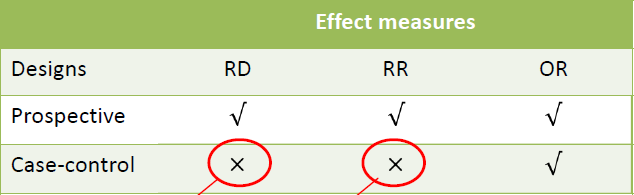
• Measures of effect for categorical data
  • Risk Difference
  • Risk Ratio
  • Odds Ratio
• Confounding and Standardization
• Mantel-Haenszel Test
• Power and Sample-Size Estimation for Stratified Categorical Data

9.1 Study Design

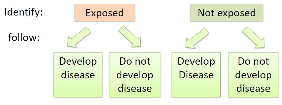
Prospective(Cohort) study: a group of disease-free individuals(Cohort) is identified at one point in time and are followed over a period of time until some of them develop the disease.(if so, the disease is related to exposure variables)

9.1.1

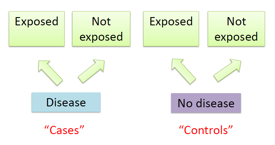
Restrospective study:

1. a group that has the disease under study (the cases)

2. a group that does not have the disease under study (the controls).

Then make an attempt to relate their prior health habits to their current disease status.

9.1.2

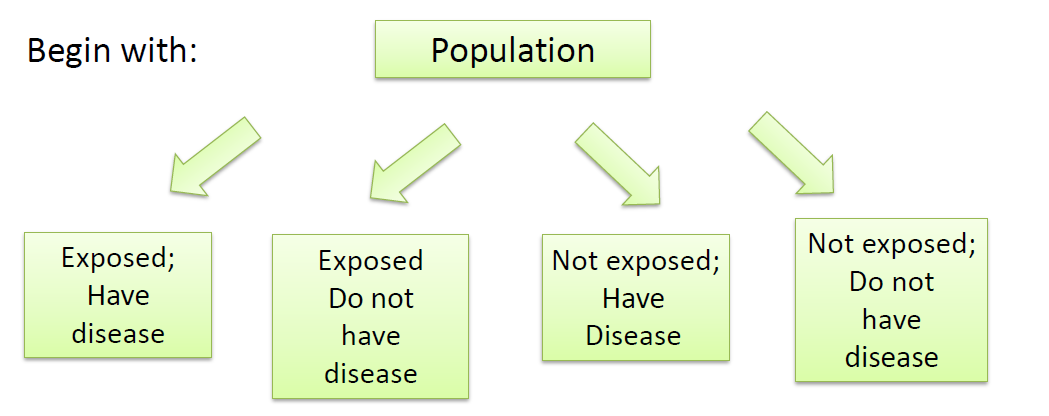
Cross-Sectional(Prevalence) study: a study population is ascertained at a single point in time.

9.1.3

9.2 Measures of effect for categorical data

9.2

9.2.1 The Risk Difference(RD)

\[RD=p_1-p_2\]

\(p_1\) = probability of developing disease for exposed individuals

\(p_2\) = probability of developing disease for unexposed individuals

Then

\[ \frac{|p_1-p_2-(\hat{p_1}-\hat{p_2})|-(\frac{1}{2n_1}+\frac{1}{2n_2})}{\sqrt{\frac{p_1q_1}{n_1}+\frac{p_2q_2}{n_2}}}\sim N(0,1) \]

Therefore, if \(p_1q_1/n_1+p_2q_2/n_2\) is approximated by \(\hat{p_1}\hat{q_1}/n_1+\hat{p_2}\hat{q_2}/n_2\), CI for \(\hat{p_1}-\hat{p_2}\) can be obtained:

\[ \hat{p_1}-\hat{p_2}-[1/(2n_1)+1/(2n_2)]\pm z_{1-\alpha/2}\sqrt{\hat{p_1}\hat{q_1}/n_1+\hat{p_2}\hat{q_2}/n_2},\text{ if }\hat{p_1}>\hat{p_2}\\ \hat{p_1}-\hat{p_2}+[1/(2n_1)+1/(2n_2)]\pm z_{1-\alpha/2}\sqrt{\hat{p_1}\hat{q_1}/n_1+\hat{p_2}\hat{q_2}/n_2},\text{ if }\hat{p_1}\leq\hat{p_2} \]

9.2.2 The Risk Ratio(RR)

\[ RR=\frac{p_1}{p_2}\Rightarrow \widehat{RR}=\frac{\hat{p_1}}{\hat{p_2}} \]

\(p_1\) = probability of developing disease for exposed individuals

\(p_2\) = probability of developing disease for unexposed individuals

To obtain the interval estimate, Delta Method is used to calculate \(Var(\ln\frac{\hat{p_1}}{\hat{p_2}})\), that is

\[ \begin{aligned} Var(\ln\widehat{RR})&=Var(\ln\hat{p_1})+Var(\ln\hat{p_2})\\ &\approx\frac{1}{\hat{p_1}^2}Var(\hat{p_1})+\frac{1}{\hat{p_2}^2}Var(\hat{p_2})\\ &=\frac{1}{\hat{p_1}^2}\frac{n_1\hat{p_1}\hat{q_1}}{n_1^2}+\frac{1}{\hat{p_2}^2}\frac{n_2\hat{p_2}\hat{q_2}}{n_2^2}\\ &=\frac{1-\hat{p_1}}{\hat{p_1}n_1}+\frac{1-\hat{p_2}}{\hat{p_2}n_2}\\ &=\frac{b}{an_1}+\frac{d}{cn_2} \end{aligned} \]

With \(se[\ln(\widehat{RR})]\), the approximate CI for \(\ln(RR)\) is given by

\[ [\ln(\widehat{RR})\pm z_{1-\alpha/2}\sqrt{\frac{b}{an_1}+\frac{d}{cn_2}}] \]

Further, the approximate CI for \(RR\) is given by

\[ [\exp\left\{\ln(\widehat{RR})\pm z_{1-\alpha/2}\sqrt{b/(an_1)+d/(cn_2)}\right\}] \]

9.2.3 The Odds Ratio(OR)

\(p\) = the probability of a success

The Odds in favor of success = \(\frac{p}{1-p}\)

then

\[ OR=\frac{p_1/q_1}{p_2/q_2}=\frac{p_1q_2}{p_2q_1} \]

which can also be calculated with the cotingency table \(OR=\frac{ad}{bc}\). OR is popularly used in study because it's comparible (why?).

Similarly, use Delta method to obtain \(Var(\ln\hat{OR})\), that is

\[ \begin{aligned} Var(\ln(\hat{OR}))&=Var(\ln\frac{\hat{p_1}}{1-\hat{p_1}})+Var(\ln\frac{\hat{p_2}}{1-\hat{p_2}})\\ &=\frac{1}{a}+\frac{1}{b}+\frac{1}{c}+\frac{1}{d} \end{aligned} \]

Then the approximate CI for \(\ln(OR)\) is given by

\[ \ln(\hat{OR})\pm z_{1-\alpha/2}\sqrt{\frac{1}{a}+\frac{1}{b}+\frac{1}{c}+\frac{1}{d}} \]

Further, the approximate CI for \(OR\) is given by

\[ \hat{OR}\exp\left\{\pm z_{1-\alpha/2}\sqrt{1/a+1/b+1/c+1/d}\right\} \]

9.2.4 Delta Method

The variance of a function of a random variable \(f(X)\) can be approximated by

\[ Var[f(X)]=[f'(X)]^2Var(X) \]

9.2.5 Comparison between RD,RR,OR

9.2.5

Suppose that a random fraction \(f_1\) of subjects with disease and a random fraction \(f_2\) of subjects without disease in the reference population are included in our study sample.(no sampling bias)

Therefore \(a=f_1A,c=f_1C,b=f_2B,d=f_2D\)

If we estimate the \(RR\) from study sample, we obtain \(\hat{RR}=\frac{a/(a+b)}{c/(c+d)}=\frac{A/(f_1A+f_2B)}{C/(f_1C+f_2D)}\), which doesn't equal to \(RR=\frac{A/(A+B)}{C/(C+D)}\), unless \(f_1=f_2\). But this is unlikely to be true because the usual sampling strategy is to oversample subjects with disease.

When estimating \(OR\), we can see that \(\hat{OR}=\frac{ad}{bc}=\frac{f_1Af_2D}{f_2Bf_1C}=\frac{AD}{BC}=OR\).

9.3 Confounding and Standardization

Confounding variable is a variable that is associated with both the disease and the exposure variable. Such a variable must usually be controlled for before looking at a disease-exposure relationship.

Stratification The analysis of disease-exposure realtionships in separate subgroups of the data, in which the subgroups are defined by one or more potential confounders.

Standardization (Age-standardized as example)

Suppose people in a study population are stratified into k age groups, the risk of disease among the exposed in the ith age group is \(\hat{p_{i1}}=\frac{x_{i1}}{n_{i1}}\) and the risk of disease among the unexposd in the ith age group is \(\hat{p_{i2}}=\frac{x_{i2}}{n_{i2}}\)

Age-standardized risk of disease among the exposed

\[ \hat{p_1}^*=\sum n_i\hat{p_{i1}}/\sum n_i \]

Age-standardized risk of disease among the unexposed

\[ \hat{p_2}^*=\sum n_i\hat{p_{i2}}/\sum n_i \]

Standardized RR:

\[ RR^*=\frac{\hat{p_{1}}^*}{\hat{p_{2}}^*} \]

9.4 Mantel-Haenszel Test

Target: test homogeneity in the various strata

9.4

1. Form \(k\) strata based on the level of the confounding variables. Construct a \(2\times 2\) table relating disease and exposure within each stratum
2. the total observed number of units (\(O\)) in the (1,1) cell over all strata \[O=\sum O_i=\sum a_i\]
3. the total expected number of units (\(E\)) in the (1,1) cell over all strata \[E=\sum E_i=\sum \frac{(a_i+b_i)(a_i+c_i)}{n_i}\]
4. Compute the variance (\(V\)) of \(O\) under \(H_0\) \[V=\sum V_i=\sum \frac{(a_i+b_i)(c_i+d_i)(a_i+c_i)(b_i+d_i)}{n_i^2(n_i-1)}\]
5. The test statistic is given by \[X_{MH}^2=\frac{(|O-E|-0.5)^2}{V}\stackrel{H_0}{\sim}\chi_1^2\]

Assuming that the underlying \(OR\) is the same for each stratum, an estimate of the common underlying \(OR\) is provided by

\[ \widehat{OR}_{MH}=\frac{\sum a_id_i/n_i}{\sum b_ic_i/n_i} \]

9.5 Woolf Method

Target: Test for homogeneity of ORs over different strata

Hypothesis: \(H_0:OR_1=...=OR_k\quad v.s. \quad H_1:OR_i\neq OR_j,\exists i,j\)

(MH test \(H_0:OR_1=...=OR_k=1\))

\(\ln\widehat{OR_i}=\ln[a_id_i/(b_ic_i)]\), denote \(w_i=(\frac{1}{a_i}+\frac{1}{b_i}+\frac{1}{c_i}+\frac{1}{d_i})^{-1}\)

\[ \overline{\ln OR}=\frac{\sum w_i\ln\widehat{OR_i}}{\sum w_i} \]

Test Statistic:

\[ \begin{aligned} X_{HOM}^2&=\sum w_i(\ln\widehat{OR_i}-\overline{\ln OR})^2\\ &=\sum w_i(\ln\widehat{OR_i})^2-\frac{(\sum w_i\ln\widehat{OR_i})^2}{\sum w_i}\stackrel{H_0}{\sim}\chi_{k-1}^2 \end{aligned} \]

9.6 Matched-pair Studies

Suppose we want to study the relationship between two variables.

\(n_A\) number of discordant pairs of type A

\(n_B\) number of discordant pairs of type B

1. MH estimator \(\widehat{OR}=n_A/n_B\)
2. \(Var(\ln\widehat{OR})=1/(n\hat{p}\hat{q}),\hat{p}=n_A/(n_A+n_B),\hat{q}=1-\hat{p}\)
3. Test statistic

\[ \frac{\ln\widehat{OR}-\ln OR}{\sqrt{1/(n\hat{p}\hat{q})}}\stackrel{H_0}{\sim}N(0,1) \]

9.7 Power and Sample-Size Estimation

(Refer to PPT)

Lecture 10 Multiple Logistic Regression

Outline:

• Multiple Logistic Regression
• Extensions to Logistic Regression
• Sample Size Calculation in Logistic Regression Model

10.1 Multiple Logistic Regression

Denote \(p\) the probability of disease, the regression model

\[ p=\alpha+\beta_1x_1+...+\beta_kx_k \]

Logit function: map \((-\infty,\infty)\rightarrow(0,1)\)

\[ logit(p)=\ln\frac{p}{1-p} \]

Then the multiple logistic-regression model is given by

\[ logit(p)=\ln\frac{p}{1-p}=\alpha+\beta_1x_1+...+\beta_kx_k \]

or equivalently

\[ p=\frac{e^{\alpha+\beta_1x_1+...+\beta_kx_k}}{1+e^{\alpha+\beta_1x_1+...+\beta_kx_k}} \]

10.1.1 Categorical variable

For a certain categorical variable(j):

\(logit(p_A)=\alpha+...+\beta_j(1)+...+\beta_kx_k\)

\(logit(p_B)=\alpha+...+\beta_j(0)+...+\beta_kx_k\)

So that \(logit(p_A)-logit(p_B)=\beta_j\Leftrightarrow\dfrac{p_A/(1-p_A)}{p_B/(1-p_B)}=e^{\beta_j}\)

\[ OR=\frac{Odds_A}{Odds_B}=e^{\beta_j} \]

CI for the true \(OR\) : \(\exp(\hat{\beta_j}\pm z_{1-\alpha/2}se(\hat{\beta_j}))\)

Note:

2X2表格，前瞻性、回顾性实验区别？

前瞻性实验：\(logit(P(Y|X))=\beta_0+\beta_1X\)

回顾性实验：\(logit(P(Y|X))=\alpha_0+\alpha_1X\)

由于\(OR\)在两组实验中相同，\(\beta_1=\alpha_1\)，考虑\(\beta_0\)和\(\alpha_0\)是否相等

在模型拟合中，截距项是一个“基准”（PPT13）而\(OR\)是一个基于基准的浮动值

\[ logit(p)=\ln\left\{\frac{p(D|E)}{1-p(D|E)}\right\}=\alpha+\beta E\\ OR=\frac{p_1/(1-p_1)}{p_0(1-p_0)}=\frac{\exp(\gamma_1)}{\exp(\gamma_0)}=e^\beta \]

在前瞻性和回顾性实验中，\(\gamma_0\)基准的含义不同，分别为\(\frac{a}{a+b}\)和\(\frac{A}{A+B}\)，因而\(\beta_0\)和\(\alpha_0\)的含义不同

由列联表可以求出患病率在暴露组(exposed)和非暴露组(unexposed)中的数值为\(\frac{a}{a+c}\)和\(\frac{b}{b+d}\)，或由逻辑回归模型有\(e^{\hat{\alpha}+\hat{\beta}}/(1+e^{\hat{\alpha}+\hat{\beta}})\)和\(e^{\hat{\alpha}}/(1+e^{\hat{\alpha}})\)

10.1.2 Continuous variable

For a certain continuous variable(j):

\(logit(p_A)=\alpha+...+\beta_j(x_j+\Delta)+...+\beta_kx_k\)

\(logit(p_B)=\alpha+...+\beta_jx_j+...+\beta_kx_k\)

then \(\widehat{OR}=e^{\hat{\beta_j}\Delta}\) relating the exposure variable to the dependent variable after controlling all other variables

CI for the true \(OR\) : \(\exp(\hat{\beta_j}\Delta\pm z_{1-\alpha/2}se(\hat{\beta_j})\Delta)\)

10.1.3 Hypothesis Testing

Target: To test whether to risk factors is statistical significance

Hypothesis: \(H_0:\beta_j=0,\beta_i\neq 0 (i\neq j)\quad v.s. \quad H_1:\beta_i\neq 0,\forall i\)

Test Statistic:

\[ z=\frac{\hat{\beta_j}}{se(\hat{\beta_j})}\stackrel{H_0}{\sim}N(0,1) \]

10.1.4 Prediction

First compute the linear predictor \(\hat{L}=\hat{\alpha}+...+\hat{\beta_k}x_k\), then the point estimate:

\[ \hat{p}=\frac{e^{\hat{L}}}{1+e^{\hat{L}}} \]

Pearson residuals:

\[ r_i=\frac{y_i-\hat{p_i}}{se(\hat{p_i})} \]

where \(y_i\) is the proportion of successes among the ith group of observations/numbers of success observations

Deviance residuals:

\[ r_i=sign(y_i-\hat{p_i})\sqrt{-2[y_i\log\hat{p_i}+(1-y_i)\log(1-\hat{p_i})]} \]

10.2 Extensions to Logistic Regression

10.2.1 Conditional Logistic Regression

Target: assess the association between two variables, but control for certain covariates denoted in summary by \(\tilde{z}\)

Subdivide the data into \(S\) matched sets (\(i=1,...,S\), a single case and \(n_i\) controls):

\[ logit(p(D_{ij}=1))=\alpha_iI(\text{in the ith set})+\beta x_{ij}+\gamma z_{ij} \]

then the conditional probability that the jth member of a matched set is a case given that there is exactly one case in the matched set, denoted by \(p_{ij}\)

\[ \begin{aligned} p_{ij}&=Pr(D_{ij}=1|\sum_{k=1}^{n_i}D_{ik}=1)\\ &=\frac{Pr(D_{ij}=1)\prod_{k\neq j}Pr(D_{ik}=0)}{\sum_lPr(D_{il}=1)\prod_{k\neq l}Pr(D_{ik}=0)}\\ &=\exp(\beta x_{ij}+\tilde{\gamma}\tilde{z_{ij}})/\sum_l\exp(\beta x_{il}+\tilde{\gamma}\tilde{z_{il}}) \end{aligned} \]

The conditional Likelihood, where \(j_i\) is the case in the ith matched set:

\[ L=\prod_{i=1}^Sp_{ij_i} \]

• for two subjects(case and control) in the ith matched set, \(\tilde{z_{ij}}=\tilde{z_{il}}\) and \(x_{ij}=x_{il}+1\)
• \(RR=Pr(D_{ij}=1)/Pr(D_{il}=1)=\exp(\beta)\)

10.2.2 Polychotomous Logistic Regression

Situation: outcome variable has more than 2 categories

\[ Pr(1st)=\frac{1}{1+\sum_{r=2}^Q\exp(\alpha_r+\sum_{k=1}^K\beta_{rk}x_k)} \]

\[ Pr(qth)=\frac{\exp(\alpha_q+\sum_{k=1}^K\beta_{qk}x_k)}{1+\sum_{r=2}^Q\exp(\alpha_r+\sum_{k=1}^K\beta_{rk}x_k)},q=2,...,Q \]

the odds of subject S is in the qth outcome category, denoted by \(Odds_{q,S}\)(compare with the control group, i.e.\(Pr(qth)/Pr(1st)\))

\[ Odds_{q,S}=\exp(\alpha_q+\sum_{k=1}^K\beta_{qk}x_k)) \]

then we can compare the \(OR\) for being in category \(q\) v.s. control group for subject A and B (suppose that A and B only differ in \(x_k\) and \(x_k+1\)):

\[ \frac{Odds_{q,A}}{Odds_{q,B}}=\exp(\beta_{qk}) \]

10.2.3 Ordinal Logsitic Regression

Target: the case of \(c(c\geq 2)\) ordered categories

\[ \log\frac{Pr(y\leq j)}{Pr(y\geq j+1)}=\alpha_j-\beta_1x_1-...-\beta_kx_k,j=1,...,c-1 \]

then we obtain

\[ (\text{odds that }y\leq j|x_q=x)/(\text{odds that }y\leq j|x_q=x-1)=e^{\beta_q} \]

10.3 Sample Size Calculation in Logistic Regression Model

10.3.1 Continuous X

\[ \log(\frac{P(Y=1|x)}{1-P(Y=1|x)})=\beta_0+\beta_1x \]

Hypothesis: \(H_0:\beta_1=0\quad v.s. \quad H_1:\beta_1\neq 0\)

If the rationale is if \(Y\) is not related to \(X\), then \(\mu_1=\mu_2\), where \(\mu_1=E(X|Y=0),\mu_2=E(X|Y=1)\)

The equivalence hypothesis testing: \(H_0:\mu_1=\mu_2\quad v.s. \quad H_1:\mu_1\neq\mu_2\)

The sample size being required for testing the equality of two independent sample means is

\[ n=\frac{(k+1)^2}{k}\cdot\frac{\sigma^2(z_{1-\alpha/2}+z_{1-\beta})^2}{(\mu_1-\mu_2)^2} \]

where \(\sigma^2\) is the common variance of two normal distributions and \(k=\frac{n_2}{n_1}=\frac{p_1}{1-p_1}\), \(p_1=Pr(Y=1|x=EX)\)

Note that \(P(Y=1|x)=\frac{f(x|Y=1)P(Y=1)}{f(x)}\), then

\[ \frac{P(Y=1|x)}{P(Y=0|x)}=\frac{f(x|Y=1)P(Y=1)}{f(x|Y=0)P(Y=0)}=\frac{\frac{1}{\sqrt{2\pi}\sigma}\exp(-\frac{(x-\mu_2)^2}{2\sigma^2})P(Y=1)}{\frac{1}{\sqrt{2\pi}\sigma}\exp(-\frac{(x-\mu_1)^2}{2\sigma^2})P(Y=0)} \]

\[ \Rightarrow\log(\frac{P(Y=1|x)}{1-P(Y=1|x)})=\log(\frac{P(Y=1)}{P(Y=0)})+\frac{(x-\mu_1)^2-(x-\mu_2)^2}{2\sigma^2} \]

so that we have \(Odds=C+\frac{\mu_2-\mu_1}{\sigma}\cdot\frac{x}{\sigma}\) and \(\beta_1=\frac{\mu_2-\mu_1}{\sigma}\) has the meaning of the \(\log OR\) when \(x\) increase to \(x+\sigma\). Thus,

\[ \begin{aligned} n&=\frac{(k+1)^2}{k}\cdot\frac{(z_{1-\alpha/2}+z_{1-\beta})^2}{(\frac{\mu_1-\mu_2}{\sigma})^2}\\ &=\frac{(z_{1-\alpha/2}+z_{1-\beta})^2}{p_1(1-p_1)\beta_1^2}\\ &=\frac{(z_{1-\alpha/2}+z_{1-\beta})^2}{p_1(1-p_1)\log(\frac{Odds_2}{Odds_1})^2} \end{aligned} \]

10.3.2 Binary X

\[ n=(1+k)\cdot\frac{(z_{1-\alpha/2}\sqrt{\frac{p(1-p)(k+1)}{k}}+z_{1-\beta}\sqrt{p_0(1-p_0)+\frac{p_1(1-p_1)}{k}})^2}{(p_0-p_1)^2} \]

where \(p_0\) and \(p_1\) are proportion that \(Y=1|X=0,1\) and \(p=\frac{p_0+kp_1}{1+k}\)

Suppose \(B\) is the proportion of the sample with \(X=1\), overall rate is \(p=(1-B)p_0+Bp_1\), then \(k=\frac{B}{1-B}\)

\[ n=\frac{(z_{1-\alpha/2}\sqrt{\frac{p(1-p)}{B}}+z_{1-\beta}\sqrt{p_0(1-p_0)+\frac{p_1(1-p_1)(1-B)}{B}})^2}{(p_0-p_1)^2(1-B)} \]

10.3.3 Multiple Logistic Regression

\[ var_p(b_1)=var_1(b)/(1-R^2) \]

where \(R^2\) is equal to the proportion of the variance of \(X_1\) explained by the regression relationship with \(X_2,...,X_p\)

\[ n_p=n_1/(1-R^2) \]

Lecture 11 Clustered Binary Data

Outline:

• Equivalence Studies
• Missing Data

11.1 Equivalence Studies

Target: test whether the "effectiveness" is enough

Denote \(p_1\) the survival rate for the standard treatment and \(p_2\) the survival rate for the experimental treatment

• Superiority test (good enough)
  • Higher means better: \(H_1:p_2>p_1+\delta\)
  • Higher means worse: \(H_1:p_2<p_1-\delta\)
• Non-inferiority test (not so bad)
  • Higher means better: \(H_1:p_2>p_1-\delta\)
  • Higher means worse: \(H_1:p_2<p_1+\delta\)

Example: \(p_1=0.8,\delta=0.1\), Non-inferiority test

\[ H_0:p_1-p_2\geq \delta \quad v.s.\quad H_1:p_2>p_1-\delta \]

\[ z^*=\frac{\hat{p_1}-\hat{p_2}-(p_1-p_2)}{\sqrt{\hat{p_1}\hat{q_1}/n_1+\hat{p_2}\hat{q_2}/n_2}}\stackrel{H_0}{\sim}N(0,1) \]

and the rejection region \(z^*<-z_{1-\alpha}\)

Sample size:

\[ \begin{aligned} 1-\beta&=Pr(\hat{p_1}-\hat{p_2}+z_{1-\alpha}\sqrt{\frac{\hat{p_1}\hat{q_1}}{n_1}+\frac{\hat{p_2}\hat{q_2}}{n_2}}\leq\delta)\\ &=Pr(z^*\leq \frac{\delta-(p_1-p_2)}{\sqrt{\hat{p_1}\hat{q_1}/n_1+\hat{p_2}\hat{q_2}/n_2}}-z_{1-\alpha})\\ &=\Phi(\frac{\delta-(p_1-p_2)}{\sqrt{\hat{p_1}\hat{q_1}/n_1+\hat{p_2}\hat{q_2}/n_2}}-z_{1-\alpha}) \end{aligned} \]

so that we have \(z_{1-\beta}=\frac{\delta-(p_1-p_2)}{\sqrt{\hat{p_1}\hat{q_1}/n_1+\hat{p_2}\hat{q_2}/n_2}}-z_{1-\alpha}\), assume that \(n_2=kn_1\), it can be shown that

\[ n_1=\frac{(\hat{p_1}\hat{q_1}+\hat{p_2}\hat{q_2}/k)(z_{1-\alpha}+z_{1-\beta})^2}{[\delta-(p_1-p_2)]^2} \]

11.2 Missing Data

Imputation: Imputation is defined as the estimation of a missing variable as a function of other covariates that are present, including the outcome

Multiple Imputation is a Monte Carlo technique in which the missing values are replaced by \(m>1\) simulated versions, where \(m\) is typically small

1. Covariates: \(x_1,...,x_k\) have complete \(x_1,...,x_{k-1}\) and missing for \(N_{mis}\) subjects in \(x_k\) and \(N_{obs}\) are available. A binary outcome \(y\)
2. Run a multiple regression analysis of \(x_k\) on \(x_1,...,x_{k-1},y\) based on the complete data \[x_k=\alpha+\gamma_1x_1+...+\gamma_{k-1}x_{k-1}+\delta y+\epsilon\]
3. For \(i=1,...,N_{mis}\) subjects with missing data on \(x_k\), calculate an estimated value for \(x_k\), denoted by \(x_{i,k,1}\) for ith subject \[\widehat{x_k}=\hat{\alpha}+\hat{\gamma_1}x_1+...+\widehat{\gamma_{k-1}}x_{k-1}+\hat{\delta}y\]
4. Denote \(\xi(X)\) a Monte Carlo sample, then \[x_{i,k,1}=\xi(\hat{\alpha})+\xi(\hat{\gamma_1})x_1+...+\xi(\widehat{\gamma_{k-1}})x_{k-1}+\xi(\hat{\delta})y+\xi\cdot MSE\]
5. Run a logistic regression \[\ln\frac{p}{1-p}=\alpha+\beta_1x_1+...+\beta_kx_k\]
6. Repeat steps 3-5 for \(m-1\) additional imputations
7. The estimates from the \(m\) seperate imputations are then combined into a overall estimate for \(\beta_j\) \[\hat{\beta_j}=\sum_{q=1}^m\frac{\hat{\beta_{j,q}}}{m}\]

The overall variance is

\[ Var(\hat{\beta_j})=\sum_{q=1}^m\frac{Var(\hat{\beta_{j,q}})}{m}+\frac{m+1}{m}\sum_{q=1}^m\frac{(\hat{\beta_{j,q}}-\hat{\beta_j})^2}{m-1} \]